ROC

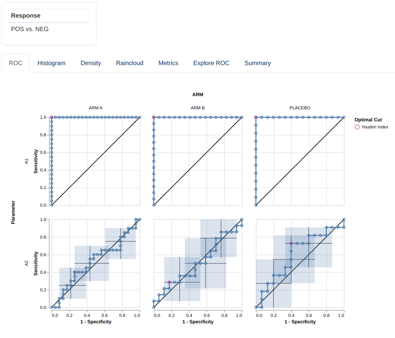
This guide provides a detailed overview of the dv.roc module and its features. It is meant to provide guidance to App Creators on creating Apps in DaVinci using the dv.roc module. Walk-throughs for sample app creation using the module are also included to demonstrate the various module specific features.

The dv.roc module makes it possible to visualize a set of ROC related charts and compare independent ROC curves for different continuous parameters with respect to a single binary endpoint. This allows a user to evaluate how predictive is a continuous parameter of binary endpoint.

Pre-requisite:

“Parameter” Term Disambiguation

The guide uses the term “parameter” at several places. This term in the guide represents clinical analysis parameters and values such as laboratory values, safety values, etc as used in the clinical dataset context. This can be confused with the word parameter as used in a programming context - “parameters of a function”. Therefore, to fully disambiguate the usage in this guide:

Parameter is used exclusively in the clinical dataset context
Argument is used to represent parameter of a function in the programming context

Features

dv.roc features the following plots:

A set of ROC curves
A set of histograms showing the distribution of the continuos parameter values
A set of probability density plots showing the distribution of the continuous parameter values
A set of raincloud plots showing the distribution of the continuous parameter values
A set of line plots showing metrics for the results of the classification
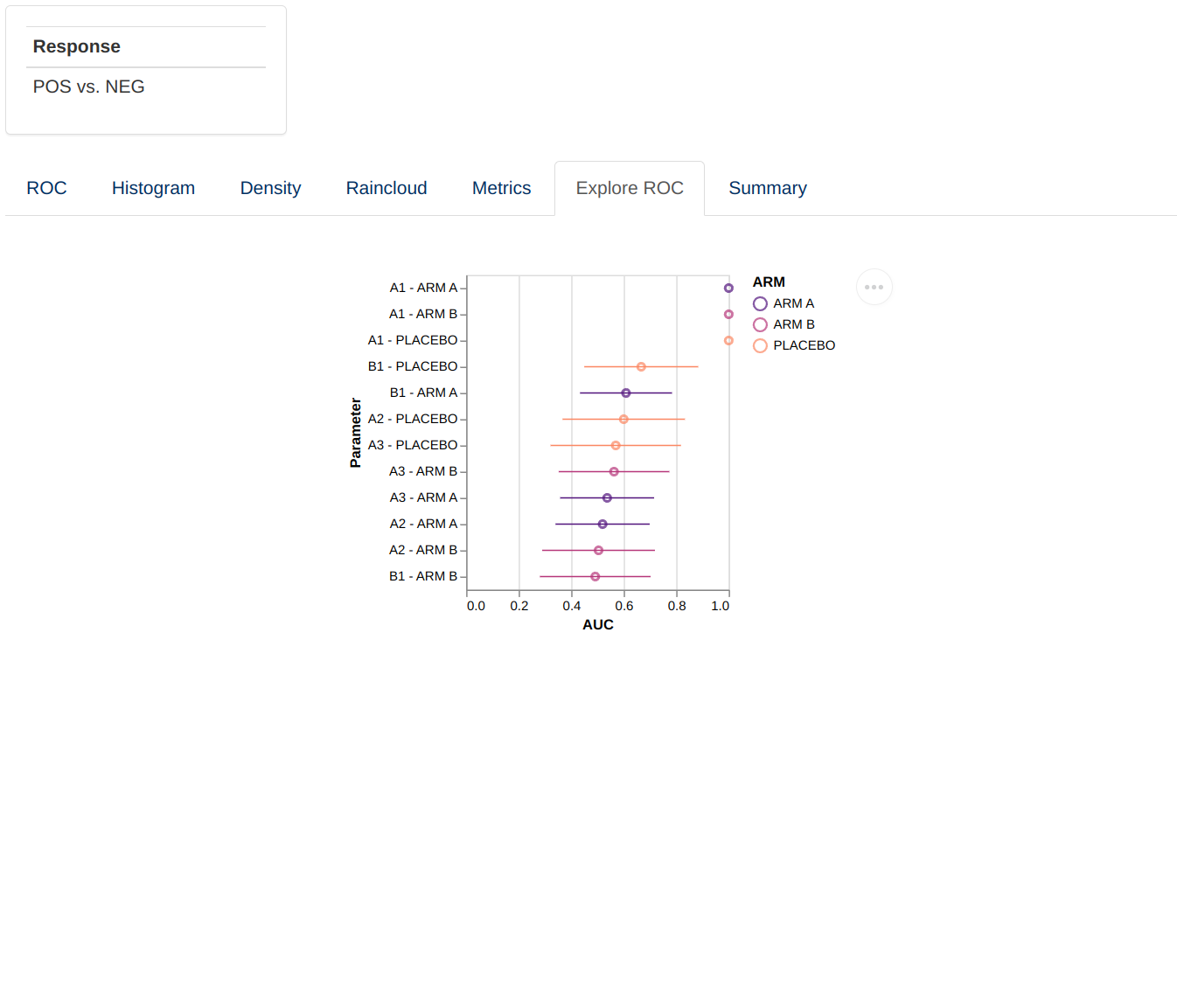
A point plot indicating the AUC for each parameter/parameter-group combination
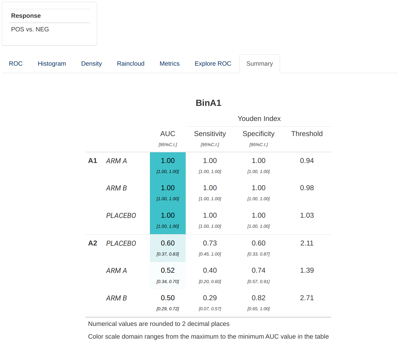
A summary table for the ROC analysis

Arguments for the module

dv.roc::mod_roc() module uses several arguments with the following being mandatory and the rest optional. As part of app creation, the app creator should specify the values for these arguments as applicable.

Mandatory Arguments

module_id : A unique identifier of type character for the module in the app.
subjid_var: A common column across all datasets that uniquely identify subjects. By default: “SUBJID”
pred_dataset_name: The name of the dataset that contains the continuous parameters to be used as predictors in the ROC analysis. It expects a dataset similar to https://www.cdisc.org/kb/examples/adam-basic-data-structure-bds-using-paramcd-80288192 , 1 record per subject per parameter per analysis visit

It expects, at least, the columns passed in the arguments, subjid_var, pred_cat_var, pred_par_var, pred_visit_var and pred_value_var.
resp_dataset_name: The name of the dataset that contains the parameters to be used as responses/binary endpoints in the ROC analysis. It expects a dataset similar to https://www.cdisc.org/kb/examples/adam-basic-data-structure-bds-using-paramcd-80288192 , 1 record per subject per parameter per analysis visit

It expects, at least, the columns passed in the arguments, subjid_var, resp_cat_var, resp_par_var, resp_visit_var and resp_value_var.
group_dataset_name: The name of the dataset that contains the variables that will be used to group plots in the module.

It expects a dataset with an structure similar to https://www.cdisc.org/kb/examples/adam-subject-level-analysis-adsl-dataset-80283806 , one record per subject It expects to contain, at least, subjid_var.

Refer to dv.roc::mod_roc() for the complete list of arguments and their description.

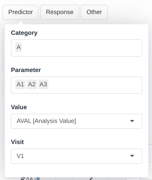
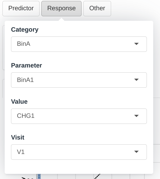
Input menus

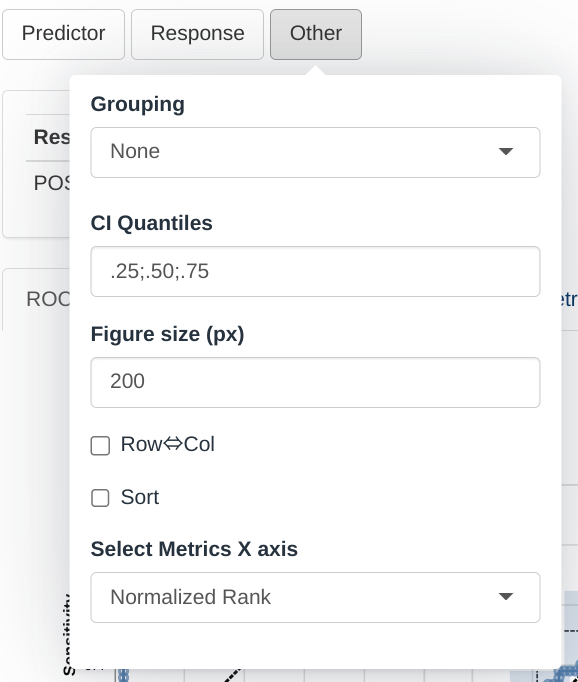A set of menus allows to select which parameters will be used as predictors for the response variable and customize the visualization in the module.

Visualizations

This visualizations consists of a facetted plot based on parameters and grouping variable. Each plot represents a ROC curve with a set of confidence intervals (as defined in Other menu)and optimal cut points (see dv.roc::compute_roc()). Hovering over the figure will show a tooltip providing additional information for each of the points.

Facetting can be replaced by a Nx4 matrix of plots sorted by AUC.

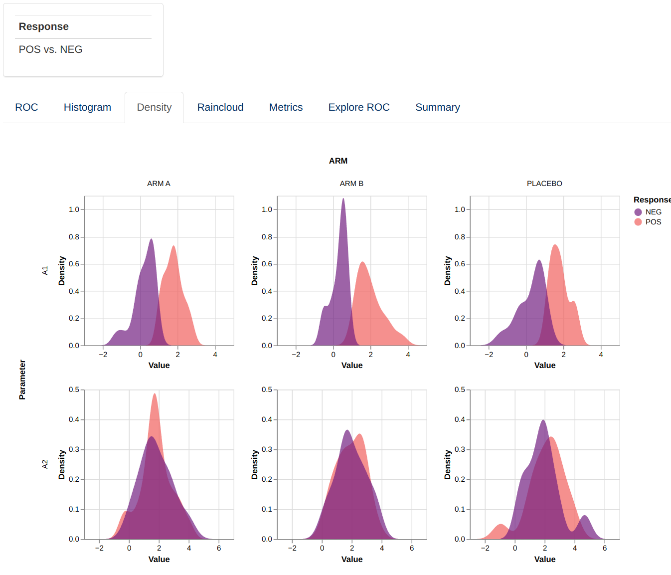
Histogram and Density

This visualizations consists of a facetted plot based on parameters and grouping variable. Each plot represents a histogram or density plot for the values of each predictor parameter grouped and colored based on the response value.

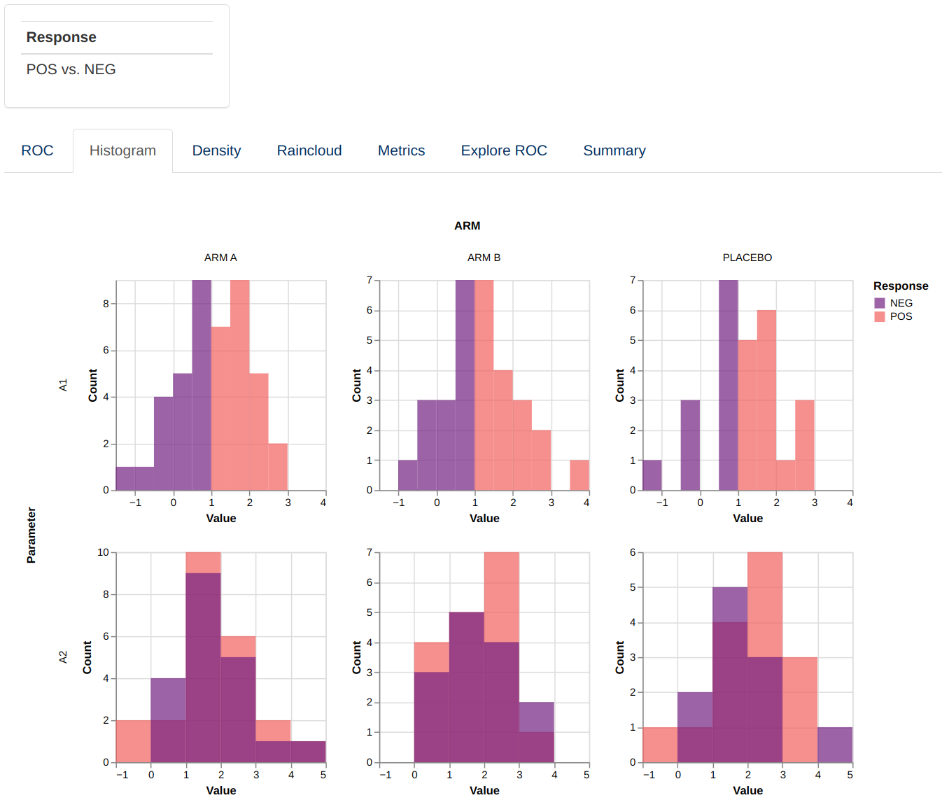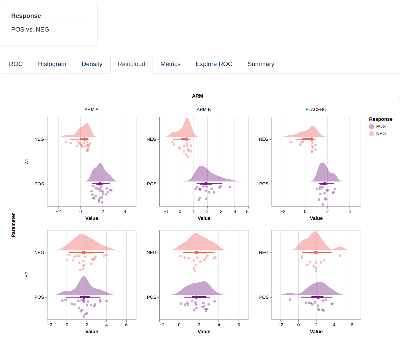
Raincloud

This visualization consists of a facetted plot based on parameters and grouping variable. Each plot represents a raincloud plot for the values of each predictor parameter grouped and colored based on the response value. The top part of the raincloud corresponds to a density plot, the bottom part correspond to individual data points, and the markes between them correspond to %5, 25%, 50%, 75% and 95% quantiles. Hovering over the figure will show a tooltip providing additional information for each of the points and markers.

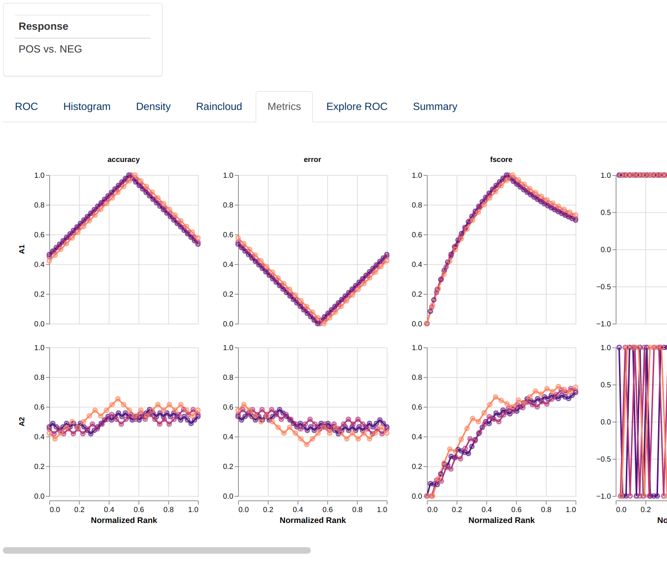
Metrics

This visualization consists of a facetted plot based on parameters and metrics and colored based on grouping. Each plot represents a line graph indicating the performance of the classification with respect to the threshold use for classification. The X axis can represent the score represented by the parameter value, raw, normalized or normalized and ranked.

Explore

This visualization consists of a sorted lineplot representing the AUC and its confidence interval per parameter, or parameter and grouping. All predictors parameters are represented regardless of the selection in the Predictor menu.

Summary

This table summarizes the results of the ROC curves and its optimal cut points.

Custom Compute Functions

This module provides the user with some default ROC analysis functions, nonetheless there are different approaches or preferences for different packages that performs this type of analysis. Additionally, because it is a data derivation, the user is provided and in charge of checking those functions and calculations. For this purpose this analysis functionality is isolated and can be modified and checked independently.

The default functions in charge of this calculations are compute_roc_data() and compute_metric_data(). But the user can create alternative functions, for example for which metrics are presented. This can be done simply by writing another function that have the same arguments and returns a similar data structure, see the documentation of the functions for further details. Two helper functions assert_compute_roc_data() and assert_compute_metric_data() can be used to check that the output of the user-defined function is correct (this checking is not exhaustive and is only prepared to catch common errors).