Multi-State Models for Oncology • oncomsm

library(oncomsm)
library(dplyr, warn.conflicts = FALSE)
library(ggplot2)

tl;dr: The multi-state characteristics of RECIST-like visit data in oncology can be exploited to reduce bias at interim analyses of objective response rate and drive event prediction for probability of success calculations.

In early oncology trials, (objective tumor) response based on the RECIST criteria is often used as primary endpoint to establish the activity of a treatment. Often, response is treated as binary variable although it is a delayed event endpoint. At the final analysis, this simplification is of little concern since all individuals tend to be followed up long enough to ignore the small amount of censoring. However, when continuously monitoring such a trial, the assumption of sufficient follow-up is no longer fulfilled at interim analyses and a simple binary analysis is biased.

The problem can be addressed by extending the statistic binary response model to a three-state model for “stable”, “response”, and “progression or death”. The respective transition numbers are given in the graph below.

Often, a hazard-based approach is used to model multi-state data. However, a hazard-based approach has several disadvantages:

The hazard scale is difficult to interpret since it is a momentary risk, not a probability. This leads to problems with prior specification in a Bayesian setting. The Bayesian approach is, however, particularly useful in the early development process since it allows to augment data with prior opinion or evidence and thus improve accuracy.
A hazard based, non-Markov multi-state model leads to intractable expressions for the implicitly given transition probabilities. Hence they need to be calculated by simulation which makes the model less convenient to work with if transition probabilities a or of primary interest. Since the (objective) response rate often plays an important role in the analysis of early oncology trials, this is a disadvantage.

An alternative framework to model multi-state data are mixture models. For details, see Jackson et al. (2022) and Jackson (2022). Here, we describe the concrete application to he simplified “stable”, “response”, “progression” model. The approach is similar to Aubel et al. (2021) and Beyer et al. (2020).

Here, a semi-Markov approach is used. This means that the time to the next transition only depends on the time already spent in a state, not on the full history of previous jumps. Additionally, it is assumed that the transition times between states conditional on both originating and target state can be described by Weibull distributions. This parametric family encompasses the exponential distribution with constant transition rates as special cases but also allows increasing or decreasing hazards over time.

Let \(\tau_{S}\) be the transition time from the “stable” state and \(\tau_{R}\) the transition tome from the “response” state (also “sojourn” times). Let further \(R\) be a binary random variable with \(R=1\) if a response occurs, then the model can be specified as:

\[ \begin{align} R &\sim \operatorname{Bernoulli}(p) \\ \tau_{S} \,|\, R = 1 &\sim \operatorname{Weibull}(k[1], \lambda[1]) \\ \tau_{S} \,|\, R = 0 &\sim \operatorname{Weibull}(k[2], \lambda[2]) \\ \tau_{R} &\sim \operatorname{Weibull}(k[3], \lambda[3]) \end{align} \] where \(k\) is the vector of shape- and \(\lambda\) the vector of scale parameters. Let further \(f_i(t)\) be the PDF of the Weibull distribution of transition \(i\in\{1,2,3\}\) as indicated in the above figure and let \(F_i(t)\) the corresponding CDF. This model implies that \[ \operatorname{Pr}\big[\,\tau_{S} > t \,\big] = p\cdot(1 - F_1(t)) + (1 - p)\cdot(1 - F_2(t))\\ \] hence, it can be seen as a mixture model.

The median of a Weibull-distributed random variable is directly related to shape and scale parameters. Since the former is more convenient to interpret, the Weibull distributions are parameterized directly via their shape and median. The scale parameter can then be recovered via the relationship

\[ \operatorname{scale} = \frac{\operatorname{median}}{\log(2)^{1/\operatorname{shape}}} . \]

The following priors are used:

a normal prior for the log-odds of response \(\operatorname{logit}(p) \sim \mathcal{N}(\mu_p,\sigma_p^2)\)
a truncated normal prior for the median of each transition \(\operatorname{median}_{\,i} \sim \mathcal{N}(\mu_i,\sigma_i^2)[\,0,\infty)\)
a flat prior on the shape of each transition \(\operatorname{shape}_{\,i} \sim \operatorname{Uniform}(a_i, b_i)\)
it is assumed that the observation process (visit spacing) is fixed, e.g. every 6 weeks. This means that all transition times are interval censored.

We treat recruitment times as independent of outcome. They can be modeled separately if required.

We assume that all times are given in months.

Specifying the model

The following code defined the prior assumptions for a two-group trial with a visit-spacing of 1.2 months, i.e., about 6 weeks.

mdl <- create_srp_model(
  # names of the arms/groups
  group_id = c("control", "intervention"),
  # per-group logodds of response|stable
  logodds_mean = c(logodds(.25), logodds(.5)),
  logodds_sd = c(.75, .75),
  # m[i,j] is the median time to next event for group i and transition j
  median_time_to_next_event = matrix(c(
    3, 2, 6,
    2, 8, 12
  ), byrow = TRUE, nrow = 2, ncol = 3),
  # fixed standard deviation of the prior for all median times
  median_time_to_next_event_sd = matrix(
    1,
    byrow = TRUE, nrow = 2, ncol = 3
  ),
  # uniform prior over the shape parameter, difficult to identify,
  # better keep it tight to avoid issues with the sampler
  shape_min = matrix(
    .75,
    byrow = TRUE, nrow = 2, ncol = 3
  ),
  shape_max = matrix(
    2,
    byrow = TRUE, nrow = 2, ncol = 3
  ),
  # the visit interval
  visit_spacing = c(1.2, 1.2)
)
# TODO: implement a nice summary / print function here

The model assumptions can be visualized by sampling from the prior.

Prior checks

First, we plot the cumulative distribution functions (CDF) of the time-to-next-event over the first 36 (months) and the CDF of the response probabilities per group. These are based on a sample drawn from the prior distribution of the model. We can re-use the same parameter sample for sampling from the prior-predictive distribution by separating the sampling from the plotting steps.

Often, the rate of progression free survival (PFS) at a particular time point is of interest. This quantity is a direct function of the model parameters. Since the simplified model does not distinguish between progression or death, we denote the combined endpoint as “progression”. \[ \begin{align} \operatorname{PFS}(t) :&= \operatorname{Pr}\big[\,\text{no progression before } t\,\big] \\ &= 1 - \operatorname{Pr}\big[\,\text{progression before } t\,] \\ &= 1 - \operatorname{Pr}\big[\,\text{progression before } t\,|\, \text{response}\,]\cdot\operatorname{Pr}\big[\,\text{response}\,] \\ &\qquad- \operatorname{Pr}\big[\,\text{progression before } t\,|\, \text{no response}\,]\cdot\operatorname{Pr}\big[\,\text{no response}\,] \\ &= 1 - p\cdot\int_0^t f_1(u) \cdot F_2(t - u) \operatorname{d}u - (1 - p)\cdot F_3(t) \ . \end{align} \] The integral arises from the need to reflect the uncertainty over the state change from “stable” to “response” on the way to “progression”. Any parameter sample thus also induces a sample of the PFS rate at any given time point and the curve of PFS rate over time corresponds to the survival function of the “progression or death” event.

smpl_prior <- sample_prior(mdl, warmup = 500, nsim = 2000, seed = 36L)

plot(mdl, dt = c(0, 36), sample = smpl_prior)

Sampling from the prior-predictive distribution

Next, we draw samples from the prior-predictive distribution of the model. We sample 100 trials with 30 individuals per arm. Here, we can re-use the sample prior sample already used for plotting.

tbl_prior_predictive <- sample_predictive(
  mdl,
  sample = smpl_prior,
  n_per_group = c(30L, 30L),
  nsim = 100,
  seed = 3423423
)

We can then run some quick checks on the sampled data, e.g., the observed response rates.

tbl_prior_predictive %>%
  filter(from == "stable") %>%
  group_by(group_id) %>%
  summarize(p_response = sum(to == "response") / n())
#> # A tibble: 2 × 2
#>   group_id     p_response
#>   <chr>             <dbl>
#> 1 control           0.250
#> 2 intervention      0.479

A crude approximation of the median transition times can be obtained from the midpoints of the censoring intervals.

tbl_prior_predictive %>%
  filter(from == "stable") %>%
  group_by(group_id, from, to) %>%
  summarize(t_jump_approx = median(t_min + t_max) / 2, .groups = "drop")
#> # A tibble: 4 × 4
#>   group_id     from   to          t_jump_approx
#>   <chr>        <chr>  <chr>               <dbl>
#> 1 control      stable progression           1.8
#> 2 control      stable response              3  
#> 3 intervention stable progression           7.8
#> 4 intervention stable response              1.8

The generated data can also be visualized in swimmer plots.

plot_mstate(mdl, tbl_prior_predictive %>% filter(iter == 1))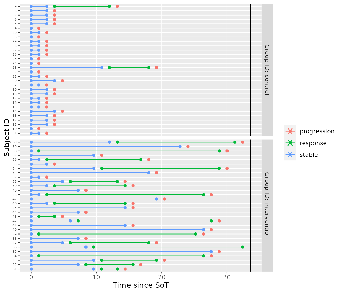

Building a visit data set

Usually, data will come in the form of individual visits, not yet in the form of interval censored transitions. We can mimic this for the sake of example by converting one of our prior predictive samples to visit data. Note that the conversion is not exact since the mstate format does not contain information about potential visits between the interval boundaries.

tbl_visits <- tbl_prior_predictive %>%
  filter(iter == 1) %>%
  mstate_to_visits(mdl, .)

print(tbl_visits)
#> # A tibble: 573 × 4
#>    subject_id group_id     t state      
#>    <chr>      <chr>    <dbl> <chr>      
#>  1 1          control    0   stable     
#>  2 1          control    1.2 stable     
#>  3 1          control    2.4 progression
#>  4 10         control    0   stable     
#>  5 10         control    1.2 progression
#>  6 11         control    0   stable     
#>  7 11         control    2.4 stable     
#>  8 11         control    3.6 progression
#>  9 12         control    0   stable     
#> 10 12         control    2.4 stable     
#> # … with 563 more rows

Next, we add recruitment times assuming an overall recruitment rate of 3 per month.

recruitment_rate_overall <- 3
# sample from poisson process
set.seed(31532)
tbl_sot <- tbl_visits %>%
  select(
    subject_id,
    group_id
  ) %>%
  distinct() %>%
  arrange(runif(n())) %>% # permute groups
  mutate(
    # poisson recruitment process
    t_sot = cumsum(rexp(n = n(), rate = recruitment_rate_overall))
  )

# add to visit times
tbl_visits <- tbl_visits %>%
  left_join(tbl_sot, by = c("subject_id", "group_id")) %>%
  mutate(t = t + t_sot) # shift event times accordingly

# convert back to mstate format and plot
tbl_visits %>%
  visits_to_mstate(start_state = "stable", absorbing_states = "progression") %>%
  plot_mstate(mdl, ., relative_to_sot = FALSE)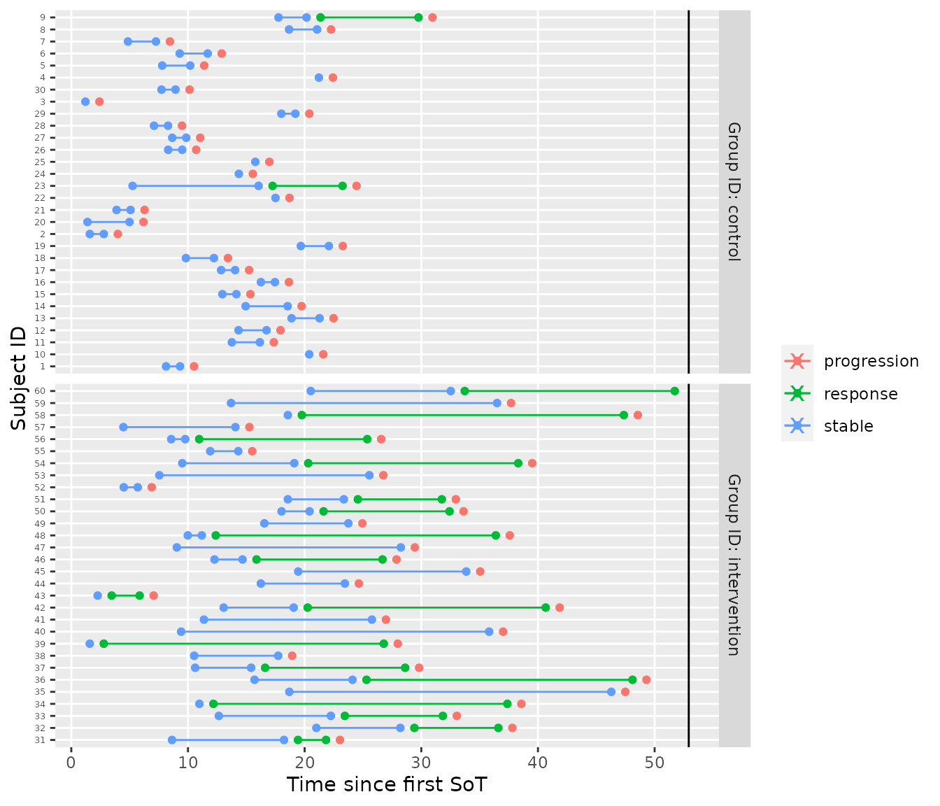

A hypothetical interim analysis

If we now cut the data at 15 months after the first SoT, we can imitate a hypothetical interim analysis.

tbl_visits_interim <- tbl_visits %>%
  filter(t <= 15)

# convert to mstate plot
tbl_mstate_interim <- visits_to_mstate(
  tbl_visits_interim,
  start_state = "stable",
  absorbing_states = "progression",
  now = 15
)
plot_mstate(mdl, tbl_mstate_interim, relative_to_sot = FALSE, now = 15)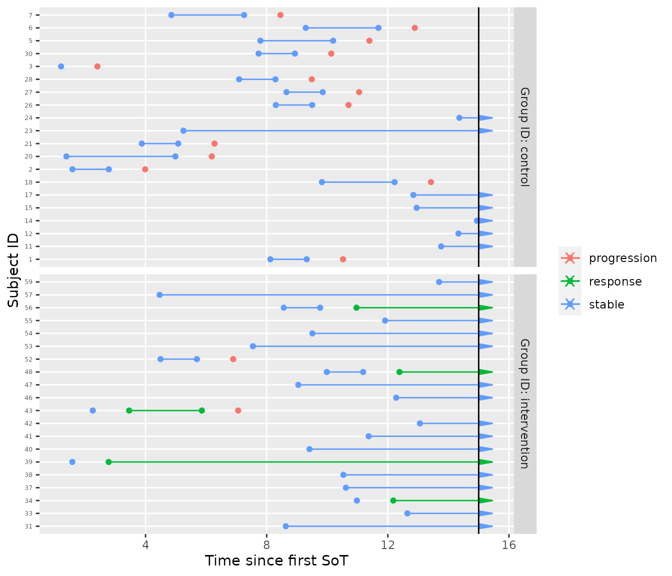

We can check the observed response rates. Careful, due to the different time-to-event these will be biased.

# estimate of the response rates (biased due to missing!)
tbl_mstate_interim %>%
  filter(from == "stable", !is.na(to)) %>%
  group_by(group_id) %>%
  summarize(p_response = sum(to == "response") / n())
#> # A tibble: 2 × 2
#>   group_id     p_response
#>   <chr>             <dbl>
#> 1 control           0    
#> 2 intervention      0.833

We can now do inference by drawing sample from the posterior distribution.

smpl_posterior <- sample_posterior(mdl, tbl_mstate_interim, seed = 76947)

plot(mdl, dt = c(0, 36), sample = smpl_posterior)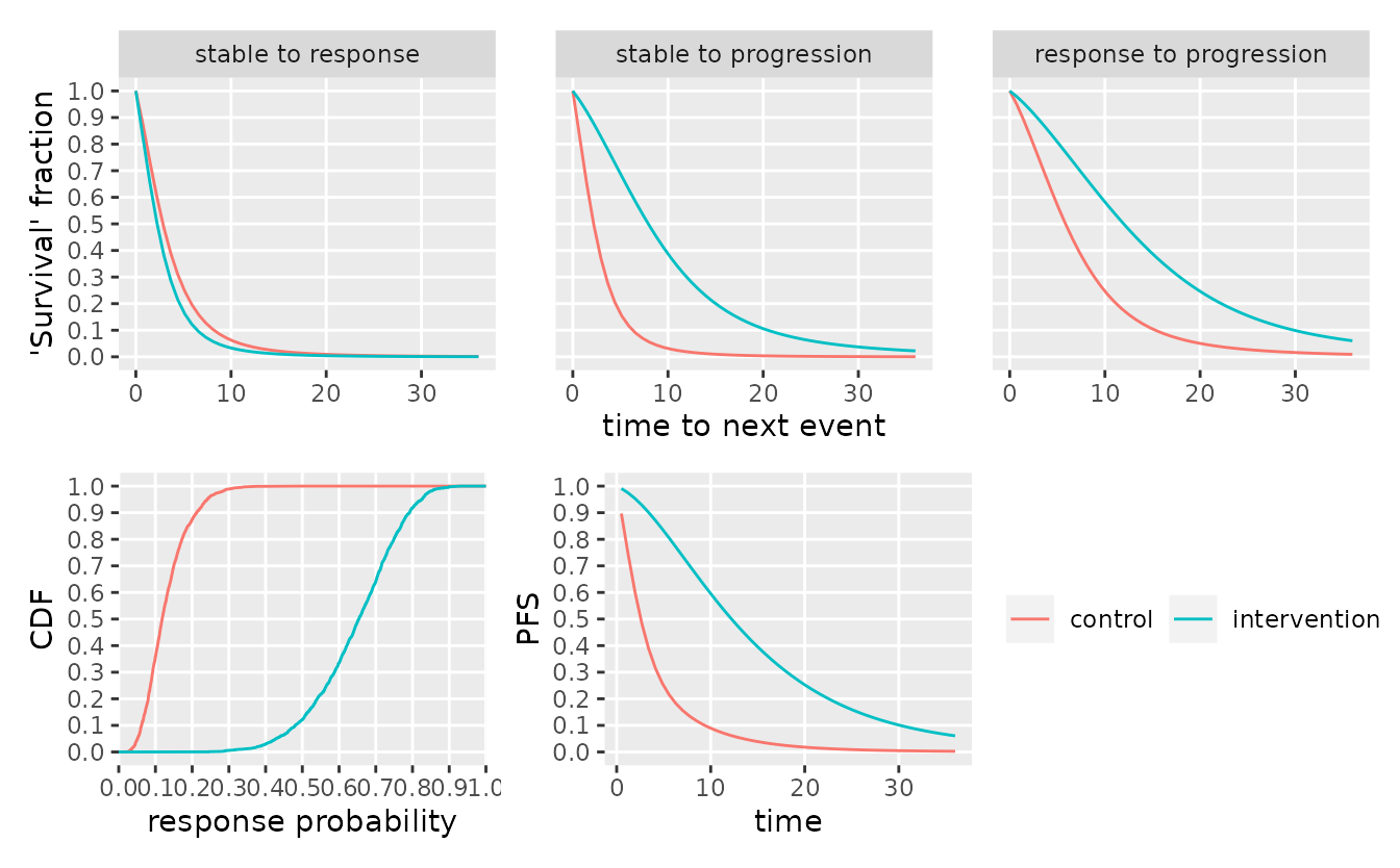


# calculate posterior quantiles of response probability
smpl_posterior %>%
  parameter_sample_to_tibble(mdl, .) %>%
  filter(parameter == "p") %>%
  group_by(group_id) %>%
  summarize(
    p_posterior_mean = median(value),
    q25 = quantile(value, probs = .25),
    q75 = quantile(value, probs = .75)
  )
#> # A tibble: 2 × 4
#>   group_id     p_posterior_mean    q25   q75
#>   <chr>                   <dbl>  <dbl> <dbl>
#> 1 control                 0.118 0.0865 0.161
#> 2 intervention            0.654 0.566  0.731

Session info

sessionInfo()
#> R version 4.2.2 (2022-10-31)
#> Platform: x86_64-pc-linux-gnu (64-bit)
#> Running under: Ubuntu 20.04.5 LTS
#> 
#> Matrix products: default
#> BLAS:   /usr/lib/x86_64-linux-gnu/blas/libblas.so.3.9.0
#> LAPACK: /usr/lib/x86_64-linux-gnu/lapack/liblapack.so.3.9.0
#> 
#> locale:
#>  [1] LC_CTYPE=C.UTF-8       LC_NUMERIC=C           LC_TIME=C.UTF-8       
#>  [4] LC_COLLATE=C.UTF-8     LC_MONETARY=C.UTF-8    LC_MESSAGES=C.UTF-8   
#>  [7] LC_PAPER=C.UTF-8       LC_NAME=C              LC_ADDRESS=C          
#> [10] LC_TELEPHONE=C         LC_MEASUREMENT=C.UTF-8 LC_IDENTIFICATION=C   
#> 
#> attached base packages:
#> [1] stats     graphics  grDevices utils     datasets  methods   base     
#> 
#> other attached packages:
#> [1] ggplot2_3.3.6      dplyr_1.0.10       oncomsm_0.1.0.9000
#> 
#> loaded via a namespace (and not attached):
#>  [1] Rcpp_1.0.9           tidyr_1.2.1          visNetwork_2.1.2    
#>  [4] prettyunits_1.1.1    ps_1.7.2             rprojroot_2.0.3     
#>  [7] digest_0.6.30        utf8_1.2.2           R6_2.5.1            
#> [10] backports_1.4.1      stats4_4.2.2         evaluate_0.17       
#> [13] highr_0.9            pillar_1.8.1         rlang_1.0.6         
#> [16] callr_3.7.3          jquerylib_0.1.4      checkmate_2.1.0     
#> [19] rmarkdown_2.17       DiagrammeR_1.0.9     pkgdown_2.0.6       
#> [22] labeling_0.4.2       textshaping_0.3.6    desc_1.4.2          
#> [25] stringr_1.4.1        htmlwidgets_1.5.4    loo_2.5.1           
#> [28] munsell_0.5.0        compiler_4.2.2       xfun_0.34           
#> [31] rstan_2.21.7         pkgconfig_2.0.3      systemfonts_1.0.4   
#> [34] pkgbuild_1.3.1       htmltools_0.5.3      tidyselect_1.2.0    
#> [37] tibble_3.1.8         gridExtra_2.3        codetools_0.2-18    
#> [40] matrixStats_0.62.0   fansi_1.0.3          crayon_1.5.2        
#> [43] withr_2.5.0          grid_4.2.2           jsonlite_1.8.3      
#> [46] gtable_0.3.1         lifecycle_1.0.3      magrittr_2.0.3      
#> [49] StanHeaders_2.21.0-7 scales_1.2.1         RcppParallel_5.1.5  
#> [52] cli_3.4.1            stringi_1.7.8        cachem_1.0.6        
#> [55] farver_2.1.1         fs_1.5.2             bslib_0.4.1         
#> [58] ellipsis_0.3.2       ragg_1.2.4           generics_0.1.3      
#> [61] vctrs_0.5.0          RColorBrewer_1.1-3   tools_4.2.2         
#> [64] glue_1.6.2           purrr_0.3.5          processx_3.8.0      
#> [67] parallel_4.2.2       fastmap_1.1.0        yaml_2.3.6          
#> [70] inline_0.3.19        colorspace_2.0-3     memoise_2.0.1       
#> [73] knitr_1.40           patchwork_1.1.2      sass_0.4.2

Aubel, Paul, Marine Antigny, Ronan Fougeray, Frédéric Dubois, and Gaëlle Saint‐Hilary. 2021. “A Bayesian Approach for Event Predictions in Clinical Trials with Time‐to‐event Outcomes.” Statistics in Medicine 40 (28): 6344–59. https://doi.org/10.1002/sim.9186.

Beyer, Ulrich, David Dejardin, Matthias Meller, Kaspar Rufibach, and Hans Ulrich Burger. 2020. “A Multistate Model for Early Decision-Making in Oncology.” Biometrical Journal 62 (3): 550–67. https://doi.org/10.1002/bimj.201800250.

Jackson, Christopher. 2022. “Flexible Parametric Multi-State Modelling with Flexsurv.” https://cran.r-project.org/web/packages/flexsurv/.

Jackson, Christopher, Brian Tom, Peter Kirwan, Sema Mandal, Shaun R Seaman, Kevin Kunzmann, Anne Presanis, and Daniela De Angelis. 2022. “A Comparison of Two Frameworks for Multi-State Modelling, Applied to Outcomes After Hospital Admissions with COVID-19.” Statistical Methods in Medical Research, July, 09622802221106720. https://doi.org/10.1177/09622802221106720.