Integration with bhmbasket

Kevin Kunzmann

library(oncomsm)
library(dplyr, warn.conflicts = FALSE)
library(future) # parallel processing
plan(multisession)

tl;dr: The bhmbasket package implements Bayesian hierarchical methods for basket trials with binary endpoints. Although oncomsm does not support hierarchical modelling, bhmbasket can be used to define ‘go’ criteria based on hierarchical models.

Start by defining a prior specification for a multi-group trial.

mdl <- create_srpmodel(
  A = define_srp_prior(
      p_mean = 0.3, p_n = 20,
      median_t_q05 = c(3, 2, 6) - 1,
      median_t_q95 = c(3, 2, 6) + 1,
      recruitment_rate = 2
    ),
  B = define_srp_prior(
      p_mean = 0.4, p_n = 20,
      median_t_q05 = c(2.5, 8, 18) - 1,
      median_t_q95 = c(2.5, 8, 18) + 1,
      recruitment_rate = 2
    ),
  C = define_srp_prior(
      p_mean = 0.5, p_n = 20,
      median_t_q05 = c(2, 12, 24) - 1,
      median_t_q95 = c(2, 12, 24) + 1,
      recruitment_rate = 2
    )
)

Defining ‘go’ decision

The bhmbasket package implements dynamic borrowing between arms in basket trials via Bayesian hierarchical models (BHMs). Here, we demonstrate how oncomsm and the prior specified in mdl can be used to derive probability of ‘go’ based on a bhmbasket analysis. We use the “Berry” type model for analysis of the response data and use a posterior \(0.25\) quantile of the response probability above \(0.3\) to declare ‘go’. This means that an individual arm is further developed if there is a \(0.75\) posterior probability according to the BHM that the response rate is larger than \(0.3\).

go <- function(model, data, nsim = 250) {
  set.seed(2340239L)
  # convert data to bhmbasket format (multi-state to binary counts)
  data <- data %>%
    group_by(group_id, subject_id) %>%
    summarize(
      responder = any(state == "response"),
      .groups = "drop_last"
    ) %>%
    summarize(
      r = sum(responder),
      n = n(),
    ) %>%
    {
      bhmbasket::createTrial(.$n, .$r)
    }
  # define Berry model in bhmbasket
  prms_berry <- bhmbasket::setPriorParametersBerry(
    mu_mean   = bhmbasket::logit(0.25),
    mu_sd     = 1,
    tau_scale = 1
  )
  # perform analysis in bhmbasket
  res <- suppressMessages(bhmbasket::performAnalyses(
    scenario_list         = data,
    method_names          = "berry",
    evidence_levels       = 1 - 0.25,
    prior_parameters_list = prms_berry,
    target_rates          = c(.2, .3, .3),
    n_mcmc_iterations     = nsim,
    verbose               = FALSE
  ))
  # 'go' if posterior quantile of response rate is sufficiently large
  return(tibble(
    group_id = model$group_id,
    go = res$scenario_1$quantiles_list$berry[[1]][5, 2:4] >= .3
  ))
}

Probability of ‘go’ before start of the trial

The ‘go’ criterion can then be applied to each of the resampled data sets.

tbl_decisions <- simulate_decision_rule(mdl,
                                        c(40, 40, 40),
                                        go,
                                        nsim = 250,
                                        seed = 32487)

tbl_pr_go_planning <- tbl_decisions %>%
  group_by(group_id) %>%
  summarize(`Pr[go] planning` = mean(go))

tbl_pr_go_planning
#> # A tibble: 3 × 2
#>   group_id `Pr[go] planning`
#>   <chr>                <dbl>
#> 1 A                    0.312
#> 2 B                    0.716
#> 3 C                    0.884

Update probability of ‘go’

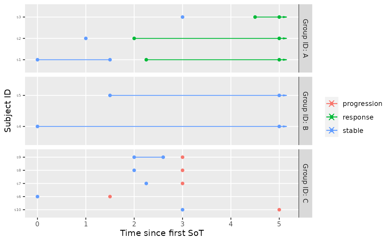
Now assume that some interim data is available. The data is fairly extreme for both group A and group B.

tbl_interim <- tribble(
   ~subject_id, ~group_id, ~t, ~state,
          "s1", "A", 0, "stable",
          "s1", "A", 1.5, "stable",
          "s1", "A", 2.25, "response",
          "s2", "A", 1, "stable",
          "s2", "A", 2, "response",
          "s3", "A", 3, "stable",
          "s3", "A", 4.5, "response",
          "s4", "B", 0, "stable",
          "s5", "B", 1.5, "stable",
          "s6", "C", 0, "stable",
          "s6", "C", 1.5, "progression",
          "s7", "C", 2.25, "stable",
          "s7", "C", 3, "progression",
          "s8", "C", 2, "stable",
          "s8", "C", 3, "progression",
          "s9", "C", 2, "stable",
          "s9", "C", 2.6, "stable",
          "s9", "C", 3, "progression",
         "s10", "C", 3, "stable",
         "s10", "C", 5, "progression"
)

# plot it
visits_to_mstate(tbl_interim, mdl) %>%
  plot_mstate(mdl, relative_to_sot = FALSE)

The prior can now be updated with this data.

smpl_prior <- sample_prior(mdl, seed = 2314513)
smpl_posterior <- sample_posterior(mdl, tbl_interim, seed = 2314)

tibble(
  group_id = mdl$group_id,
  prior = rstan::extract(smpl_prior, "p")[[1]] %>% colMeans(),
  posterior = rstan::extract(smpl_posterior, "p")[[1]] %>% colMeans()
)
#> # A tibble: 3 × 3
#>   group_id prior posterior
#>   <chr>    <dbl>     <dbl>
#> 1 A        0.302     0.391
#> 2 B        0.399     0.377
#> 3 C        0.500     0.401

The probability of ‘go’ is then updated by sampling forward from the posterior predictive.

tbl_decisions_interim <- simulate_decision_rule(
  mdl,
  c(40, 40, 40),
  go,
  data = tbl_interim,
  nsim = 250,
  seed = 32487
)

tbl_pr_go_planning %>%
  left_join(
    tbl_decisions_interim %>%
    group_by(group_id) %>%
    summarize(
      `Pr[go] interim` = mean(go)
    ),
    by = "group_id"
  )
#> # A tibble: 3 × 3
#>   group_id `Pr[go] planning` `Pr[go] interim`
#>   <chr>                <dbl>            <dbl>
#> 1 A                    0.312            0.644
#> 2 B                    0.716            0.64 
#> 3 C                    0.884            0.54