
Introduction to the 'tipmap' package
Tipping point analysis for clinical trials that employ Bayesian dynamic borrowing
Christian Stock
2024-04-04
Source:vignettes/introduction.Rmd
introduction.RmdPurpose of the package
The R package tipmap implements a tipping point analysis for clinical trials that employ Bayesian dynamic borrowing of a treatment effect from external evidence via robust meta-analytic predictive (MAP) priors. A tipping point analysis allows to assess how much weight on the informative component of a robust MAP prior is needed to conclude that the investigated treatment is efficacious, based on the total evidence. The package mainly provides an implementation of a graphical approach proposed by Best et al. (2021) for different one-sided evidence levels (80%, 90%, 95%, 97.5%).
Tipping point analyses can be useful both at the planning and the analysis stage of a clinical trial that uses external information. At the planning stage, they can help to determe (pre-specify) a weight of the informative component of the MAP prior for a primary analysis. Various possible results of the planned trial in the target population and implications for the treatment effect estimate and statistical inferences based on the total evidence may be explored for a range of weights. Through this exercise, in addition to other criteria, decision-makers can develop a sense under which circumstances they would still feel comfortable to establish efficacy with a specific level of certainty. A preferred primary weight will typically be a compromise between the belief in the applicability of the data and operating characteristics of the resulting design specifications. At the analysis stage, tipping point analyses can be used as a sensitivity analysis to assess the dependency of the treatment effect estimate and statistical inferences on the weight of the informative component of the MAP prior. This can also be understood in the sense of a reverse-Bayes analysis (Held et al. (2022)).
This vignette shows an exemplary application of the tipping point analysis with hypothetical data.
Further functions in this package (not illustrated in this vignette) facilitate the specification of a robust MAP prior via expert elicitation, specifically the choice of a primary weight (using the roulette method).
Intended use of the tipmap-package is the planning, analysis and interpretation of (small) clinical trials in pediatric drug development, where extrapolation of efficacy, often through Bayesian methods, has become increasingly common (Gamalo et al. (2022); ICH (2022); Ionan et al. (2023); Travis et al. (2023)). For an application, see Maher et al. (2024).
For the implementation of the MAP prior approach, including computation of the posterior distribution, the RBesT-package is used (Weber et al. (2021)).
Generating data for an exemplary tipping point analysis
In this vignette, we assume that results from three clinical trials conducted in adult patients (the source population) are available, which share key features with a new trial among pediatric patients (the target population). For example, they had been conducted in the same indication, studied the same drug and provided results on an endpoint of interest for the target population. This means a certain degree of exchangeability between the trials in the source and target population can be assumed. The similarity in disease and response to treatment between source and target population always need to be carefully considered in any setting, usually by clinical experts in the disease area.
We assume that it is supported by medical evidence and now planned to consider the trials in adult patients in a Bayesian dynamic borrowing approach, and we would like to create a robust MAP prior (Schmidli et al. (2014)). The treatment effect measure of interest is assumed to be a mean difference between a treated group and a control group with respect to a continuous endpoint.
Derivation of MAP prior based on trials in the source population
We start by specifying an object that contains the prior data.
The function create_prior_data() takes vectors of total
sample sizes, treatment effect estimates and their standard errors as
arguments and generates a data frame. A study label is optional.
> library(tipmap)
> prior_data <- create_prior_data(
+   n_total = c(160, 240, 320),
+   est = c(1.16, 1.43, 1.59),
+   se = c(0.46, 0.35, 0.28)
+ )
> print(prior_data)
# study_label n_total est se
# 1 Study 1 160 1.16 0.46
# 2 Study 2 240 1.43 0.35
# 3 Study 3 320 1.59 0.28We then generate a MAP prior from our prior data using the RBesT-package (Weber et al. (2021)).
> set.seed(123)
> uisd <- 5.42
> map_mcmc <- RBesT::gMAP(
+   formula = cbind(est, se) ~ 1 | study_label,
+   data = prior_data,
+   family = gaussian,
+   weights = n_total,
+   tau.dist = "HalfNormal",
+   tau.prior = cbind(0, uisd / 16),
+   beta.prior = cbind(0, uisd)
+   )
A few additional specifications are needed to be made to fit the MAP
prior model; for details see Neuenschwander and
Schmidli (2020) or Weber et al.
(2021). The variable uisd here represents an assumed
unit-information standard deviation and the specification of the prior
on between-trial heterogeneity parameter tau follows recommendations to
consider moderate heterogeneity for a two-group parameter, such as the
mean difference (Neuenschwander and Schmidli
(2020)).
This is a summary of the fitted model based on samples from the posterior distribution:
> summary(map_mcmc)
# Heterogeneity parameter tau per stratum:
#         mean    sd    2.5%   50% 97.5%
# tau[1] 0.205 0.162 0.00761 0.168 0.603
#
# Regression coefficients:
#             mean   sd  2.5%  50% 97.5%
# (Intercept) 1.43 0.25 0.922 1.44  1.92
#
# Mean estimate MCMC sample:
#            mean   sd  2.5%  50% 97.5%
# theta_resp 1.43 0.25 0.922 1.44  1.92
#
# MAP Prior MCMC sample:
#                 mean    sd  2.5%  50% 97.5%
# theta_resp_pred 1.43 0.356 0.661 1.44   2.1
A forest plot of the Bayesian meta-analysis is shown in Figure 1. It is augmented with meta-analytic shrinkage estimates per trial. The figure shows the per-trial point estimates (light point) and the 95% frequentist confidence intervals (dashed line) and the model derived median (dark point) and the 95% credible interval of the meta-analytic model.
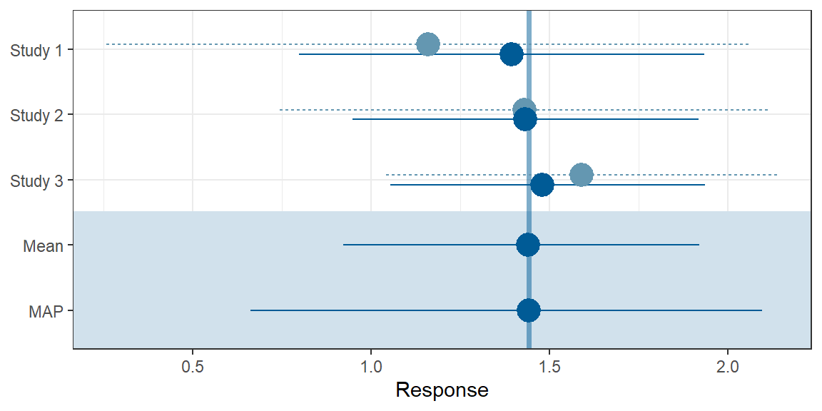
Figure 1: Forest plot.
Subsequently, the MAP prior is approximated by a mixture of conjugate normal distributions. The parametric form facilitates the computation of posteriors when the MAP prior is combined with results from the trial in the target population.
> map_prior <- RBesT::automixfit(
+   sample = map_mcmc,
+   Nc = seq(1, 4),
+   k = 6,
+   thresh = -Inf
+   )
The approximation yields a mixture of two normals:
> print(map_prior)
# EM for Normal Mixture Model
# Log-Likelihood = -1335.201
#
# Univariate normal mixture
# Reference scale: 5.298722
# Mixture Components:
#   comp1     comp2
# w 0.7717324 0.2282676
# m 1.4522222 1.3625788
# s 0.2508704 0.5793548
The density of the parametric mixture together with a histogram of
MCMC samples from the map_mcmc object is shown in Figure
2.
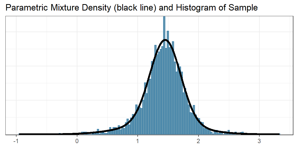
Figure 2: Overlay of the MCMC histogram of the MAP prior and the fitted parametric mixture approximation.
The derivation of the MAP prior is now complete. For normal likelihoods the parametric representation by a mixture of normals can be used to calculate posterior distributions analytically.
Trial results in the target population
We now create a numeric vector with data on pediatric trial (the total sample size, the treatment effect estimate and its standard error). In the planning stage, this may be an expected result.
> print(pediatric_trial)
#     n_total        mean          se       q0.01      q0.025       q0.05
# 30.00000000  1.02000000  1.40000000 -2.23688702 -1.72394958 -1.28279508
#        q0.1        q0.2       q0.25        q0.5       q0.75        q0.8
# -0.77417219 -0.15826973  0.07571435  1.02000000  1.96428565  2.19826973
#        q0.9       q0.95      q0.975       q0.99
#  2.81417219  3.32279508  3.76394958  4.27688702
The function create_new_trial_data() computes quantiles,
assuming normally distributed errors. This is merely used to plot a
confidence interval for the treatment effect estimate obtained in the
target trial in the tipping point plot.
Performing the tipping point analysis
Computation of posteriors for a range of weights
We can now compute posterior distributions for a range of weights
using the function create_posterior_data().
> posterior <- create_posterior_data(
+   map_prior = map_prior,
+   new_trial_data = pediatric_trial,
+   sigma = uisd)
> head(posterior, 4)
# weight q0.01 q0.025 q0.05 q0.1 q0.2 q0.25
# w=0 0.000 -2.197193 -1.700552 -1.273414 -0.7809595 -0.1846242 0.04189379
# w=0.005 0.005 -2.187599 -1.689612 -1.261009 -0.7663718 -0.1663690 0.06195571
# w=0.01 0.010 -2.178066 -1.678733 -1.248665 -0.7518369 -0.1481464 0.08192592
# w=0.015 0.015 -2.168591 -1.667913 -1.236379 -0.7373439 -0.1299534 0.10185010
# q0.5 q0.75 q0.8 q0.9 q0.95 q0.975 q0.99
# w=0 0.9562020 1.870510 2.097028 2.693363 3.185818 3.612956 4.109597
# w=0.005 0.9830598 1.855910 2.080570 2.678945 3.173427 3.602017 4.100003
# w=0.01 1.0088455 1.842214 2.064425 2.664604 3.161099 3.591139 4.090470
# w=0.015 1.0334528 1.829396 2.048622 2.650338 3.148831 3.580320 4.080995> tail(posterior, 4)
# weight q0.01 q0.025 q0.05 q0.1 q0.2 q0.25
# w=0.985 0.985 0.3713404 0.6388480 0.8437628 1.017064 1.174189 1.226884
# w=0.99 0.990 0.3832902 0.6451026 0.8468235 1.018361 1.174756 1.227315
# w=0.995 0.995 0.3949008 0.6512286 0.8498686 1.019639 1.175316 1.227742
# w=1 1.000 0.4061874 0.6572285 0.8528261 1.020899 1.175870 1.228164
# q0.5 q0.75 q0.8 q0.9 q0.95 q0.975 q0.99
# w=0.985 1.423876 1.613789 1.661732 1.793835 1.916689 2.046120 2.246768
# w=0.99 1.424005 1.613712 1.661591 1.793427 1.915776 2.044136 2.241692
# w=0.995 1.424132 1.613636 1.661451 1.793023 1.914875 2.042187 2.236725
# w=1 1.424259 1.613560 1.661313 1.792624 1.913986 2.040272 2.231867The resulting data frame has 201 rows and 14 columns. The weights increase incrementally in steps of 0.005 from 0 to 1, i.e. posterior quantiles for 201 weights are computed. For each weight the data frame contains the following 13 posterior quantiles.
> colnames(posterior)[-1]
#  [1] "q0.01"  "q0.025" "q0.05"  "q0.1"   "q0.2"   "q0.25"  "q0.5"   "q0.75"
#  [9] "q0.8"   "q0.9"   "q0.95"  "q0.975" "q0.99"
These posterior quantiles can be directly used for inferences based on the total evidence (new data and prior combined). They reflect one-sided 99%, 97.5%, 95%, 90%, 80%, and 50% evidence levels for a given weight, respectively.
Creating the tipping point plot
The function to produce the tipping point plot is called
tipmap_plot(), it requires a dataframe with data on all
components generated by the function
create_tipmap_data().
> tipmap_data <- create_tipmap_data(
+   new_trial_data = pediatric_trial,
+   posterior = posterior,
+   map_prior = map_prior)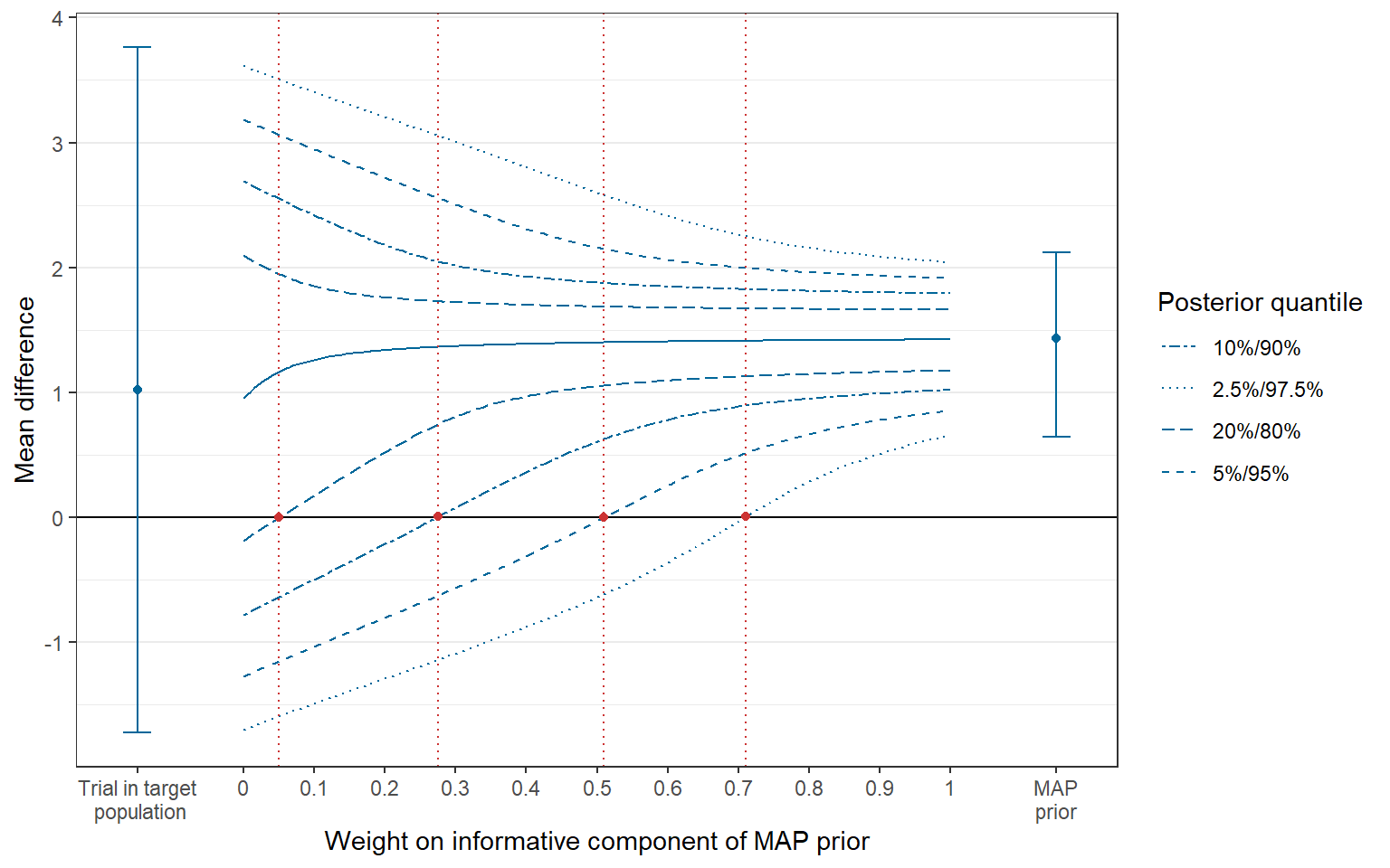
Figure 3: Tipping point plot.
At the center of the plot, quantiles of the posterior distribution are shown, defining credible intervals of the effect estimate and also one-sided evidence-levels for given weights of the informative component of the MAP prior. The intersections between the lines connecting the respective quantiles and the horizontal line at 0 (the null effect) are referred to as tipping points (indicated by vertical lines in red color). They indictae the minimum weight that is required to conclude that the treatment is efficacious for a given one-sided evidence level (Best et al. (2021)). On the left and right side of the plot, the treatment effect estimate obtained in the trial in the (pediatric) target population (with 95% confidence interval) and the MAP prior (with 95% credible interval) are shown, respectively.
The plot is a ggplot-object that can be modified
accordingly. For example, if we had chosen a primary weight of 0.38, we
could add a vertical reference line at this position. There are
additional features to customize the plot in the
tipmap_plot() function, see
help(tipmap_plot).
> primary_weight <- 0.38
> (p2 <- p1 + ggplot2::geom_vline(xintercept = primary_weight, col="green4"))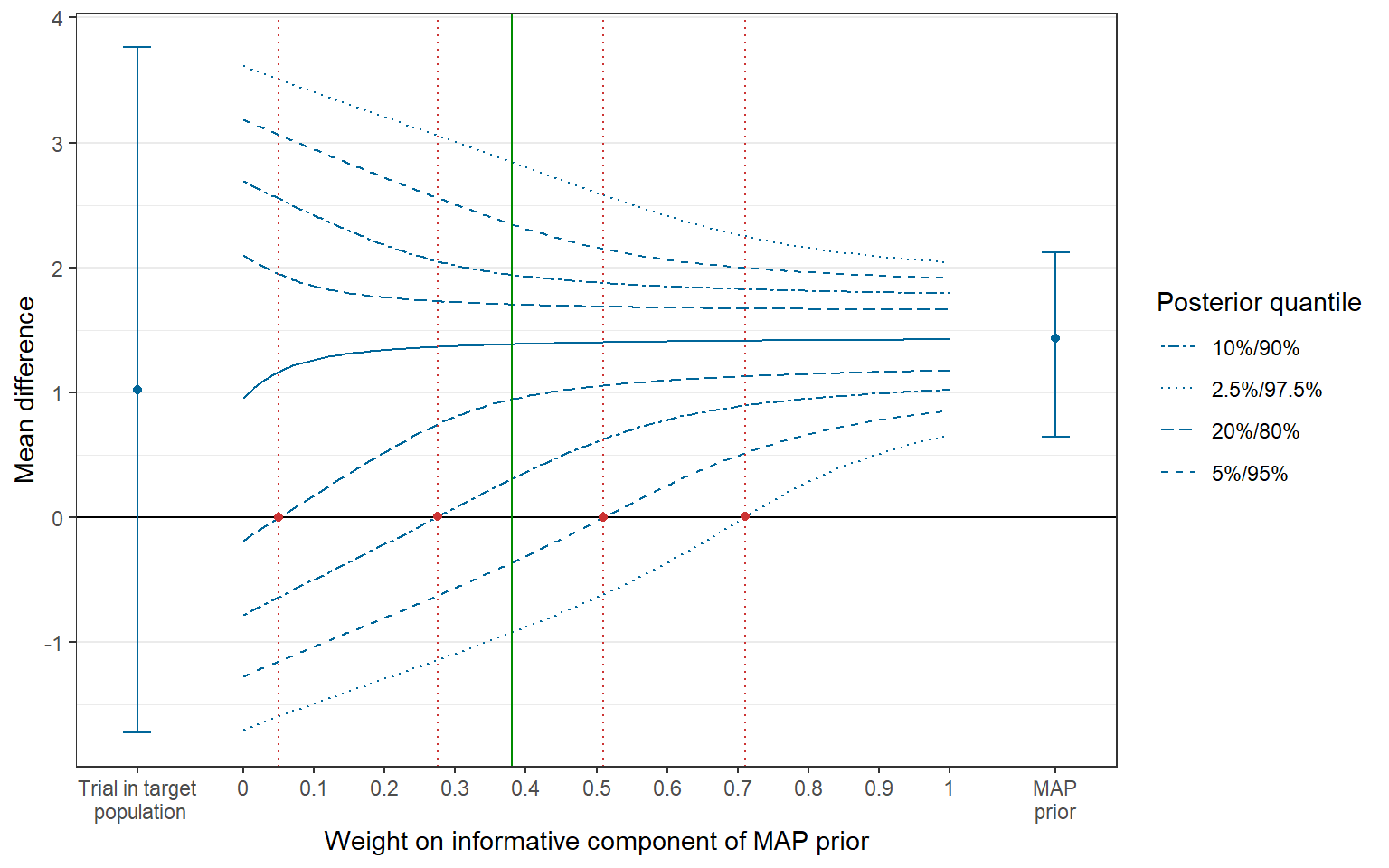
Figure 4: Tipping point plot with reference line.
We see from Figure 4 that, for a weight of 0.38, there is a probability of larger than 90% but less than 95% based on the posterior distribution that the treatment effect is larger than 0, i.e. the treatment is efficacious.
Extracting quantities of interest
The data frame with posteriors for all weights can be filtered to
obtain posterior quantiles for weights of specific interest by the
function get_posterior_by_weight():
> get_posterior_by_weight(
+   posterior = posterior,
+   weight = c(primary_weight)
+   )
#            q0.01     q0.025      q0.05      q0.1      q0.2    q0.25     q0.5
# w=0.38 -1.532189 -0.9215547 -0.3613189 0.3085641 0.9449431 1.074658 1.386163
#           q0.75     q0.8    q0.9    q0.95  q0.975    q0.99
# w=0.38 1.636538 1.704554 1.94267 2.348325 2.84356 3.444927
The function get_tipping_points() extracts tipping
points for one-sided 80%, 90%, 95% and 97.5% evidence levels,
respectively.
> tipp_points <- get_tipping_points(
+   tipmap_data = tipmap_data,
+   quantile = c(0.2, 0.1, 0.05, 0.025)
+ )
> tipp_points
#   q0.2   q0.1  q0.05 q0.025
#  0.050  0.275  0.510  0.710
Calculating the precise posterior probability that treatment effect exceeds a threshold value is possible via functions in the RBesT-package.
> prior_primary <- RBesT::robustify(
+   priormix = map_prior,
+   weight = (1 - primary_weight),
+   m = 0,
+   n = 1,
+   sigma = uisd
+   )
> posterior_primary <- RBesT::postmix(
+ priormix = prior_primary,
+ m = pediatric_trial["mean"],
+ se = pediatric_trial["se"]
+ )The posterior probability that the treatment effect is larger than 0, 0.5 and 1, respectively, can be assessed through the cumulative distribution function of the posterior.
> round(1 - RBesT::pmix(posterior_primary, q = 0), 3)
# [1] 0.927
> round(1 - RBesT::pmix(posterior_primary, q = 0.5), 3)
# [1] 0.879
> round(1 - RBesT::pmix(posterior_primary, q = 1), 3)
# [1] 0.782
This is illustrated by a cumulative density curve of the posterior.
> library(ggplot2)
> plot(posterior_primary, fun = RBesT::pmix) +
+   scale_x_continuous(breaks = seq(-1, 2, 0.5)) +
+   scale_y_continuous(breaks = 1-c(1, 0.927, 0.879, 0.782, 0.5, 0),
+                      limits = c(0,1),
+                      expand = c(0,0)
+                      ) +
+   ylab("Cumulative density of posterior with w=0.38") +
+   xlab("Quantile") +
+   geom_segment(aes(x = 0,
+                    y = RBesT::pmix(mix = posterior_primary, q = 0),
+                    xend = 0,
+                    yend = 1),
+                col="red") +
+   geom_segment(aes(x = 0.5,
+                    y = RBesT::pmix(mix = posterior_primary, q = 0.5),
+                    xend = 0.5,
+                    yend = 1),
+                col="red") +
+   geom_segment(aes(x = 1,
+                    y = RBesT::pmix(mix = posterior_primary, q = 1),
+                    xend = 1,
+                    yend = 1),
+                col="red") +
+   theme_bw()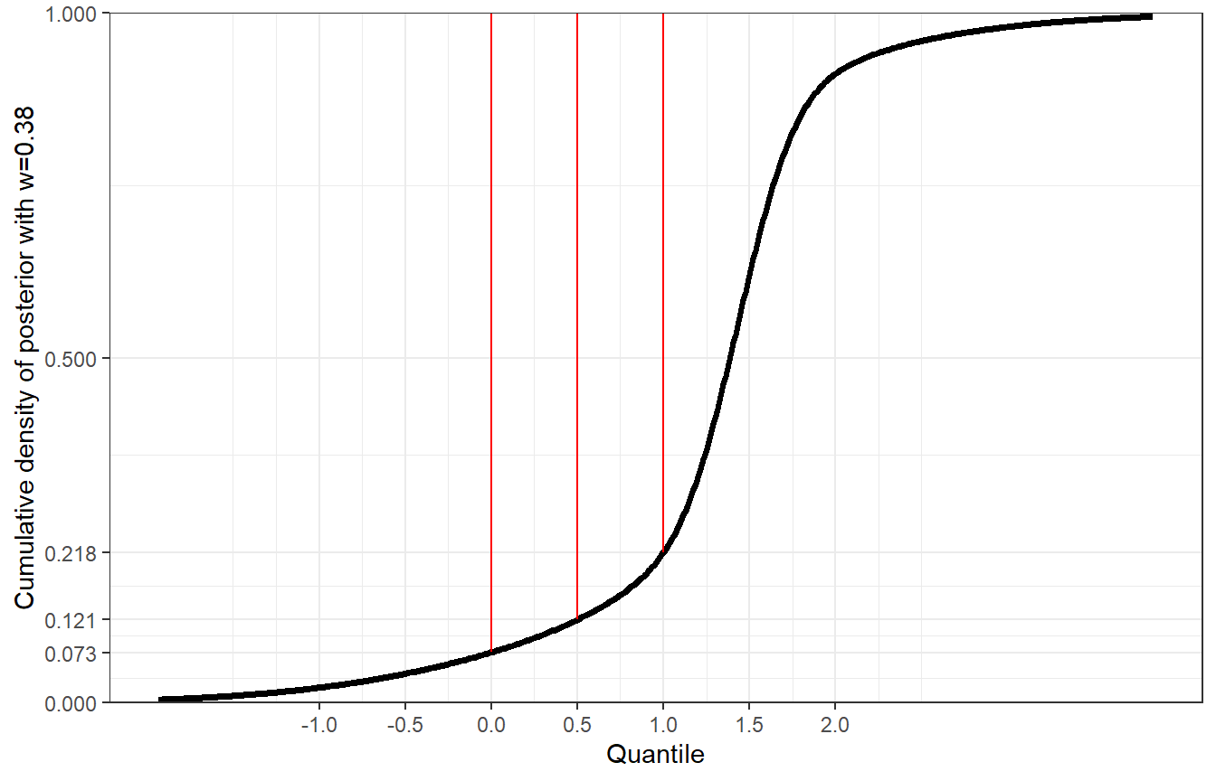
Figure 5: Cumulative density of posterior with weight w=0.38.
As a further example, for the weight corresponding to the tipping point of the one-sided evidence-level of 95% (=0.51), we would obtain a posterior probability of 95% that the treatment effect is larger than 0.
> prior_95p <- RBesT::robustify(
+   priormix = map_prior,
+   weight = (1 - tipp_points[3]),
+   m = 0,
+   n = 1,
+   sigma = uisd
+   )