Specifying a primary weight of the informative prior component

Introduction

In a clinical trial project that uses Bayesian dynamic borrowing via meta-analytic predictive (MAP) priors, ideally a pre-specified weight of the informative component of the MAP prior needs to be determined (Ionan et al. (2023)). Expert elicitation is a way through which expert judgement can be formally considered for statistical inference and decision making and it can be used to determine this weight.

For reviews on expert elicitaton see e.g. Brownstein et al. (2019) and O’Hagan (2019), and for experiences with expert elicitation in drug development see e.g. Dallow et al. (2018).

The Sheffield elicitation framework (SHELF) is an established framework that is used for the conduct of expert elicitation (O’Hagan (2019), Gosling (2018), Best et al. (2020)), and the SHELF package is available to facilitate implementation in R (The Sheffield Elicitation Framework (2019)).

This vignette provides a brief description of how expert elicitation can be used in a Bayesian borrowing analysis using robust MAP priors. It is not a description of the expert elicitation process, it shows how elicited data can be processed. It is based on and closely resembles functions in the SHELF package, but is much more limited, in the sense that it only considered determination of one weight parameter (a variable on the scale [0,1]).

The data in this example are hypothetical data.

Loading the tipmap package and set.seed:

> library(tipmap)
> set.seed(123)

Expert weightings collected using the roulette method

Here, the expert data are assumed to be collected via the ‘roulette method’ (Gosling (2018), Dallow et al. (2018)). The experts are asked to place 10 chips into a grid to create histogram-like data that reflects their preferred weighting. No particular shape of symmetry is needed.

Data from a single expert:

> chips_1exp <- c(1, 3, 4, 2, 0, 0, 0, 0, 0, 0)
> sum(chips_1exp)
# [1] 10

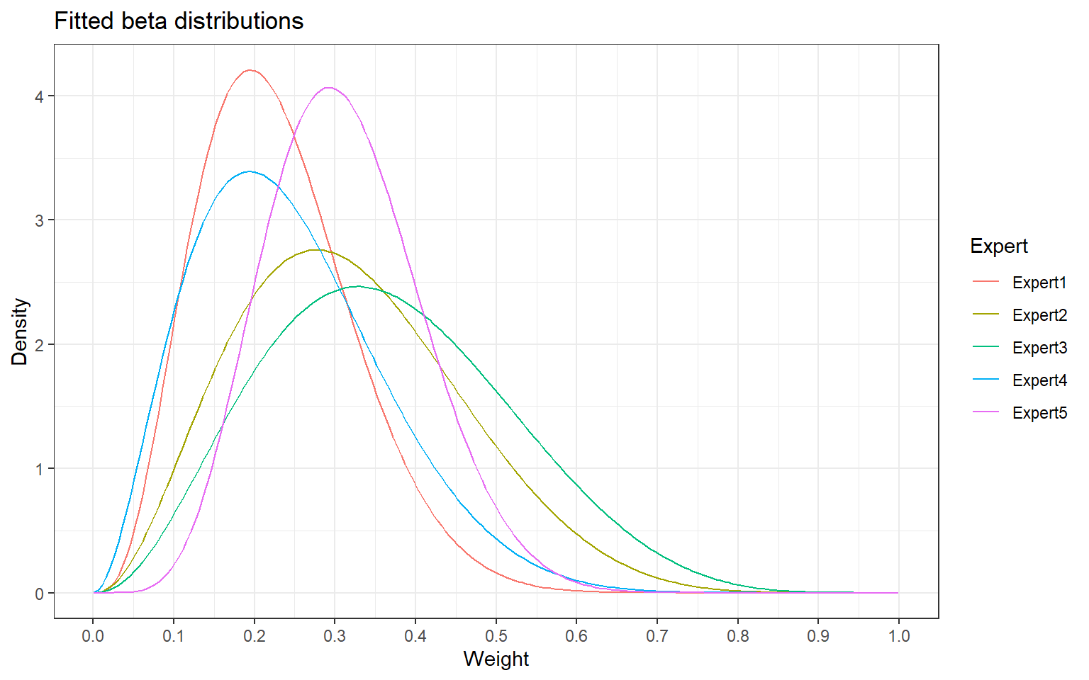
Fitting beta distributions to expert data

The roulette data are assumed to follow a beta distribution. The following calculation and fitting of a beta distribution is similar to an implementation in SHELF::fitdist and yields identical results.

Data from a single expert:

> # Compute cumulative probabilities
> (x <- get_cum_probs_1exp(chips_1exp))
#  [1] 0.1 0.4 0.8 1.0 1.0 1.0 1.0 1.0 1.0 1.0
> # Compute model inputs
> (y <- get_model_input_1exp(x))
#     w cum_probs
# 1 0.1       0.1
# 2 0.2       0.4
# 3 0.3       0.8
# 4 0.4       1.0
> # Fit beta distribution
> (fit_1exp <- fit_beta_1exp(df = y)$par)
#     alpha      beta 
#  4.195173 14.182162

For multiple experts the individual steps are handled by the fit_beta_mult_exp-function:

> chips_mult <- rbind(
+   c(1, 3, 4, 2, 0, 0, 0, 0, 0, 0),
+   c(0, 2, 3, 2, 2, 1, 0, 0, 0, 0),
+   c(0, 1, 3, 2, 2, 1, 1, 0, 0, 0),
+   c(1, 3, 3, 2, 1, 0, 0, 0, 0, 0),
+   c(0, 1, 4, 3, 2, 0, 0, 0, 0, 0)
+ )
> beta_fits <- fit_beta_mult_exp(
+   chips_mult = chips_mult
+ )
> beta_fits
#  [38;5;246m# A tibble: 5 × 4 [39m
#   alpha  beta    error convergence
#    [3m [38;5;246m<dbl> [39m [23m  [3m [38;5;246m<dbl> [39m [23m     [3m [38;5;246m<dbl> [39m [23m  [3m [38;5;246m<lgl> [39m [23m      
#  [38;5;250m1 [39m  4.20 14.2  0.001 [4m7 [24m [4m9 [24m  TRUE       
#  [38;5;250m2 [39m  3.29  6.97 0.001 [4m3 [24m [4m6 [24m  TRUE       
#  [38;5;250m3 [39m  3.30  5.70 0.003 [4m9 [24m [4m9 [24m  TRUE       
#  [38;5;250m4 [39m  2.99  9.25 0.000 [4m1 [24m [4m0 [24m [4m6 [24m TRUE       
#  [38;5;250m5 [39m  6.90 15.3  0.001 [4m3 [24m [4m6 [24m  TRUE

Summary statistics

Summary statistics for a single expert:

> (alpha <- fit_1exp[1]); (beta <- fit_1exp[2])
#    alpha 
# 4.195173
#     beta 
# 14.18216
> 
> # Mean
> (beta_mean <- alpha/(alpha+beta))
#     alpha 
# 0.2282797
> 
> # Standard deviation
> beta_sd <- sqrt( (alpha*beta)/( (alpha+beta)^2 *(alpha+beta+1) ) )
> beta_sd
#     alpha 
# 0.0953491
> 
> # Mean absolute deviation around the mean
> beta_mad_mean <- (2*(alpha^alpha)*(beta^beta))/( beta(alpha, beta) * (alpha+beta)^(alpha+beta+1) )
> beta_mad_mean
#      alpha 
# 0.07648378
> 
> # Mode
> if (alpha > 1 & beta >1) beta_mode <- (alpha-1)/(alpha+beta-2)
> if (alpha > 1 & beta >1) beta_mode <- 0.5
> beta_mode
# [1] 0.5
> 
> # Quantiles
> qbeta(p = c(0.001, 0.025, 0.05, 0.1, 0.5, 0.9, 0.95, 0.975, 0.99),
+       shape1 = alpha, shape2 = beta)
# [1] 0.03030170 0.07286831 0.08986138 0.11249422 0.21827787 0.35769286 0.40104115
# [8] 0.43928844 0.48403929
> 
> # Samples
> x <- rbeta(n = 10^6, shape1 = alpha, shape2 = beta)
> mean(x)
# [1] 0.228191
> sd(x)
# [1] 0.09536257

Summary statistics for data from multiple experts:

> expert_samples <- draw_beta_mixture_nsamples(
+   n = 10^3, 
+   chips_mult = chips_mult
+ ) 
> summary(expert_samples)
#    Min. 1st Qu.  Median    Mean 3rd Qu.    Max. 
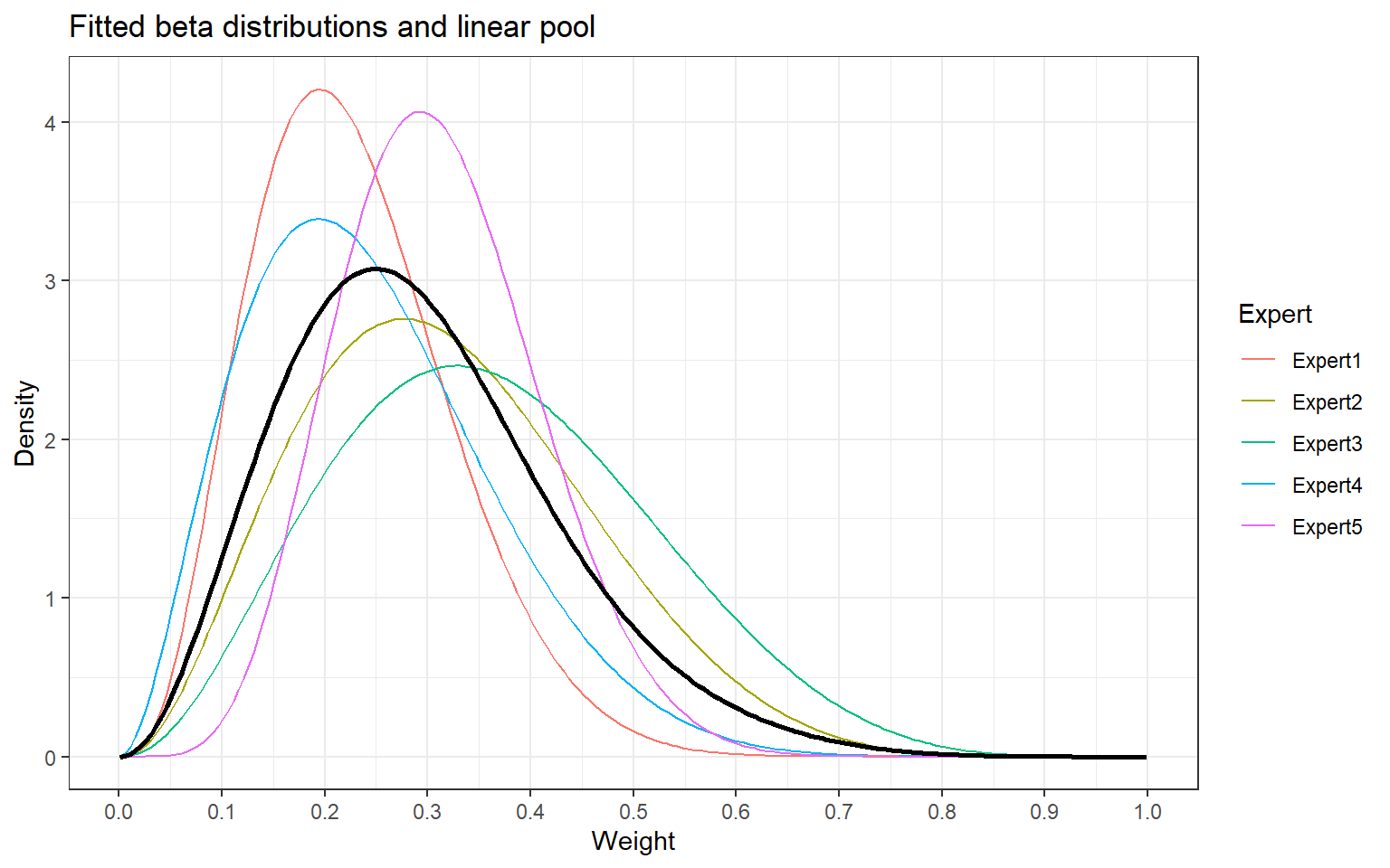
# 0.03643 0.19375 0.27175 0.28619 0.35947 0.75872

> (mean_w <- round(mean(expert_samples), 2))
# [1] 0.29

Mean or median values of the pooled distribution may be used as primary weights of the informative component of the robust MAP prior when pre-specifying the Bayesian analysis.

Figures

> # Load libraries
> packages <- c("magrittr", "ggplot2", "tibble", "dplyr")
> invisible(lapply(packages, library, character.only = T))

Without linear pooling

> # Create matrix
> fits_mat <- as.matrix(beta_fits[,c(1,2)])
> # Wide format
> fit_beta_mult_plot_wide <- tibble::tibble(
+  x = seq(0.001, 0.999, length = 200),
+  Expert1 = dbeta(x, fits_mat[1,1], fits_mat[1,2]),
+  Expert2 = dbeta(x, fits_mat[2,1], fits_mat[2,2]),
+  Expert3 = dbeta(x, fits_mat[3,1], fits_mat[3,2]),
+  Expert4 = dbeta(x, fits_mat[4,1], fits_mat[4,2]),
+  Expert5 = dbeta(x, fits_mat[5,1], fits_mat[5,2])
+ )
> # Long format
> fit_beta_mult_plot_long <- fit_beta_mult_plot_wide %>%
+   tidyr::pivot_longer(
+     !x,
+     names_to = "Expert",
+     values_to = "dens")

> # Plot without linear pool
> fig_betas_1 <- ggplot(
+   data = fit_beta_mult_plot_long,
+   aes(x = x, y = dens, goup = Expert)
+   ) +
+   geom_line(aes(color = Expert)) +
+  ggtitle("Fitted beta distributions") +
+  xlab("Weight") + ylab("Density") +
+  scale_x_continuous(breaks = c(0, 1, 2, 3, 4, 5, 6, 7, 8, 9, 10) / 10) +
+  theme_bw()
> print(fig_betas_1)

With linear pooling

> # Wide format
> fit_beta_mult_plot_wide2 <- fit_beta_mult_plot_wide %>%
+   mutate(linpool = (Expert1 + Expert2 + Expert3 + Expert4 + Expert5)/5)
> # Long format
> fit_beta_mult_plot_long2 <- fit_beta_mult_plot_wide %>%
+   tidyr::pivot_longer(
+     !x,
+     names_to = "Expert",
+     values_to = "dens")

> # Plot
> fig_betas_2 <- ggplot(
+   data = fit_beta_mult_plot_long2,
+   aes(x = x, y = dens, group = Expert)) +
+   geom_line(aes(color = Expert ) ) +
+   ggtitle("Fitted beta distributions and linear pool") +
+   xlab("Weight") + ylab("Density") +
+   scale_x_continuous(breaks=c(0,1,2,3,4,5,6,7,8,9,10)/10) +
+   theme_bw() +
+   geom_line(data = fit_beta_mult_plot_wide2,
+             aes(x = x, y = linpool, group = 1),
+             linewidth=1)
> print(fig_betas_2)

References

Best, N., Dallow, N. and Montague, T. (2020) Prior Elicitation. In: Lesaffre E, Baio G, Boulanger B (editors). Bayesian Methods in Pharmaceutical Research. CRC Press.

Brownstein, N. C., Louis, T. A., O’Hagan, A., et al. (2019) The role of expert judgment in statistical inference and evidence-based decision-making. Am Stat, 73, 56–68.

Dallow, N., Best, N. and Montague, T. H. (2018) Better decision making in drug development through adoption of formal prior elicitation. Pharm Stat, 17, 301–316.

Gosling, J. P. (2018) SHELF: The Sheffield Elicitation Framework. In Elicitation: The Science and Art of Structuring Judgement (eds L. C. Dias, A. Morton, and J. Quigley), pp. 61–93. Springer International Publishing.

Ionan, A. C., Clark, J., Travis, J., et al. (2023) Bayesian Methods in Human Drug and Biological Products Development in CDER and CBER. Ther Innov Regul Sci, 57, 436–444. DOI: 10.1007/s43441-022-00483-0.

O’Hagan, A. (2019) Expert Knowledge Elicitation: Subjective but Scientific. Am Stat, 73, 69–81. Taylor & Francis.

The Sheffield Elicitation Framework (2019) URL: Http://www.tonyohagan.co.uk/shelf/SHELF4.html, version 4.

Christian Stock

2024-04-04