library(rxsim)
library(dplyr)
library(purrr)
library(tidyr)
library(ggplot2)Example 6: Two arm | Fixed vs group-sequential design | Continuous | design comparison
two-arm
group-sequential
fixed design
continuous
design comparison
operating characteristics
A design table mapped with purrr::pmap compares a fixed single-look design against a 2-look O’Brien-Fleming group-sequential design on type-I error, power, early-stopping probability, and expected sample size.
A fixed single-look design and a group-sequential (GS) design with an early-stopping rule achieve similar type-I error and power, but the GS design can stop early under the alternative, spending fewer patients on average. This example compares the two side-by-side using a design table (a tibble where each row is a design) mapped with purrr::pmap. The approach enumerate multiple trial strategies, and scales naturally to more designs or scenarios.
Unique focus: design-table pattern, purrr::pmap over a scenario grid, 2-look O’Brien-Fleming group-sequential, operating characteristics (type-I, power, early-stop probability, expected N).
Design table
Each row in designs specifies one trial design: the look fractions and the corresponding nominal two-sided p-value boundary at each look.
# OBF K=2, equal info (0.5, 1.0), two-sided alpha = 0.05.
# Swap gsDesign::gsDesign() for other spending functions.
designs <- tibble(
  design = c("Fixed", "GS-OBF"),
  looks  = list(1.0, c(0.5, 1.0)),
  bounds = list(0.05, c(0.00517, 0.04800))
)
designs
#> # A tibble: 2 × 3
#>   design looks     bounds
#>   <chr>  <list>    <list>
#> 1 Fixed  <dbl [1]> <dbl [1]>
#> 2 GS-OBF <dbl [2]> <dbl [2]>
Fixed performs a single final analysis at full enrollment (fraction = 1.0) with two-sided alpha = 0.05. GS-OBF adds an interim at 50% information with O’Brien-Fleming spending: the interim bound is tight (p < 0.00517), spending almost no alpha early, while the final bound (p < 0.04800) is only fractionally narrower than the fixed design’s. Together the two bounds preserve overall α ≈ 0.05.
Scenario
sample_size <- 100
arms        <- c("pbo", "trt")
allocation  <- c(1, 1)
n_reps      <- 1000   # replicates per scenario row

# Block accrual: 10 subjects per time unit.
# Interim (50 enrolled) fires at t = 5; final (100 enrolled) at t = 10.
enroll_fn  <- function(n) { a <- ceiling(seq_len(n) / 10); c(a[1], diff(a)) }
dropout_fn <- function(n) rep(0, n)

# Null (no effect) and alternative (delta = 0.5 SD): design comparison, not a sweep.
scenarios <- expand_grid(design = designs$design, delta = c(0, 0.5)) |>
  left_join(designs, by = "design") |>
  mutate(seed = 1000L + row_number())
scenarios
#> # A tibble: 4 × 5
#>   design delta looks     bounds     seed
#>   <chr>  <dbl> <list>    <list>    <int>
#> 1 Fixed    0   <dbl [1]> <dbl [1]>  1001
#> 2 Fixed    0.5 <dbl [1]> <dbl [1]>  1002
#> 3 GS-OBF   0   <dbl [2]> <dbl [2]>  1003
#> 4 GS-OBF   0.5 <dbl [2]> <dbl [2]>  1004
expand_grid produces one row per (design × truth) combination; left_join attaches the looks and bounds list-columns from the design table. A seed column makes each run reproducible independently.
Populations
mk_pops <- function(delta) list(
  pbo = function(n) data.frame(id = 1:n, value = rnorm(n),        readout_time = 0),
  trt = function(n) data.frame(id = 1:n, value = rnorm(n, delta), readout_time = 0)
)
Analysis generators
mk_gens builds one named analysis per look fraction. Each fires a t-test on all subjects enrolled so far.
mk_gens <- function(looks) {
  gens <- lapply(looks, function(fr) list(
    trigger  = enroll_trigger(fr, sample_size),
    analysis = function(df, current_time) {
      e <- subset(df, !is.na(enroll_time))
      data.frame(frac = fr, n = nrow(e), p = t.test(value ~ arm, data = e)$p.value)
    }
  ))
  names(gens) <- paste0("look_", seq_along(looks))
  gens
}
enroll_trigger(fr, sample_size) fires once when enrolled count reaches fr × sample_size. The GS design registers two conditions (look_1 at n = 50, look_2 at n = 100); the Fixed design registers one (look_1 at n = 100).
Simulate
run_one runs n_reps replicates for one scenario row. After collecting results it applies the per-look boundary vector element-wise, p[k] < bounds[k], to find the first look where the trial crosses its threshold. n_used is the sample size at that look, or the full 100 if no boundary is crossed.
run_one <- function(design, delta, looks, bounds, seed) {
  set.seed(seed)
  tr <- replicate_trial(
    design, sample_size, arms, allocation, enroll_fn, dropout_fn,
    mk_gens(looks), mk_pops(delta), n = n_reps
  )
  invisible(run_trials(tr))

  per <- collect_results(tr) |>
    arrange(replicate, frac) |>
    group_by(replicate) |>
    summarise(
      first_rej = { i <- which(p < bounds); if (length(i)) min(i) else NA_integer_ },
      n_used    = if (is.na(first_rej)) last(n) else n[first_rej],
      .groups   = "drop"
    )

  tibble(
    design      = design,
    scenario    = if (delta == 0) "null (d=0)" else sprintf("alt (d=%.1f)", delta),
    reject_h0   = mean(!is.na(per$first_rej)),
    # Early stop = rejects at an interim look (first_rej < last look); always 0 for Fixed.
    early_stop  = mean(!is.na(per$first_rej) & per$first_rej < length(looks)),
    expected_n  = mean(per$n_used)
  )
}

oc <- pmap(scenarios, run_one) |> list_rbind()
For the Fixed design bounds is the scalar 0.05, so which(p < 0.05) on a single p-value. For GS-OBF bounds is c(0.00517, 0.04800) and p is a length-2 vector, so the comparison is element-wise: interim bound at look 1, final bound at look 2.
Results
oc
#> # A tibble: 4 × 5
#>   design scenario    reject_h0 early_stop expected_n
#>   <chr>  <chr>           <dbl>      <dbl>      <dbl>
#> 1 Fixed  null (d=0)      0.043      0          100
#> 2 Fixed  alt (d=0.5)     0.72       0          100
#> 3 GS-OBF null (d=0)      0.051      0.004       99.8
#> 4 GS-OBF alt (d=0.5)     0.716      0.138       93.1
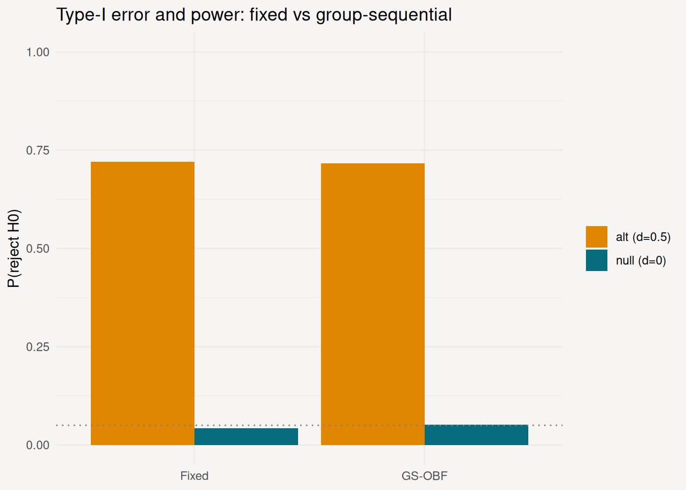
Both designs control type-I error near 0.05 and reach similar power under delta = 0.5. The GS design’s expected N drops below 100 under the alternative because some replicates stop at the interim when early evidence is compelling.
Operating characteristics
ggplot(oc, aes(design, reject_h0, fill = scenario)) +
  geom_col(position = "dodge") +
  geom_hline(yintercept = 0.05, linetype = 3, colour = "grey50") +
  coord_cartesian(ylim = c(0, 1)) +
  scale_fill_manual(values = c("#e18600", "#076d7e")) +
  labs(
    x     = NULL,
    y     = "P(reject H0)",
    fill  = NULL,
    title = "Type-I error and power: fixed vs group-sequential"
  )
knitr::kable(
  oc,
  digits  = c(0, 0, 3, 3, 1),
  col.names = c("Design", "Scenario", "P(reject H0)", "P(stop early)", "Expected N"),
  caption = "Operating characteristics: type-I error, power, early-stopping probability, and expected sample size."
)| Design | Scenario | P(reject H0) | P(stop early) | Expected N |
|---|---|---|---|---|
| Fixed | null (d=0) | 0.043 | 0.000 | 100.0 |
| Fixed | alt (d=0.5) | 0.720 | 0.000 | 100.0 |
| GS-OBF | null (d=0) | 0.051 | 0.004 | 99.8 |
| GS-OBF | alt (d=0.5) | 0.716 | 0.138 | 93.1 |
The power chart confirms both designs control type-I error near 0.05 and deliver comparable power. The table shows the GS design’s payoff: expected N drops below 100 under the alternative because some replicates stop at the interim when early evidence is compelling, while the Fixed design always uses all 100 patients.
Next steps
- Example 1: the minimal fixed design this GS design extends
- Example 4: Bayesian Go/No-Go, a different decision framework
- Conditions and Triggers: multi-look designs in depth