# Core simulation framework
library(rxsim)

# Bayesian borrowing utilities
library(RBesT)

# Helpers
library(dplyr)
library(ggplot2)

set.seed(777)Example 4: Two-arm | Fixed design | Single continuous endpoint | Bayesian Go/No-Go with placebo borrowing
two-arm
fixed design
continuous
Bayesian
Go/No-Go
borrowing
Bayesian Go/No-Go with historical placebo borrowing via
RBesT::robustify; OC curve across true effects.
Early development trials often face small sample sizes where borrowing information from historical placebo data can increase efficiency and reduce required sample size. This example demonstrates a Bayesian Go/No-Go decision rule for a Phase IIa trial, where the placebo posterior is informed by historical data via a robust mixture prior, and the treatment posterior uses a non-informative prior. A “Go” decision is issued when the posterior probability of a meaningful treatment effect (delta > threshold) exceeds a predefined threshold.
Unique focus: Bayesian Go/No-Go criterion, historical data borrowing via RBesT::robustify(), Go probability as a function of true effect size.
The setup pattern stays aligned with Example 1, while the analysis is replaced by a Bayesian decision rule with borrowing.
Scenario
A two-arm, fixed design trial (placebo vs treatment) with a single continuous endpoint and a single final analysis.
- Placebo arm uses historical borrowing through an informative prior derived from historical placebo data and robustified with a non-informative component.
- Treatment arm uses a non-informative prior.
- Go/No-Go rule: Go if P(mu_T - mu_P > delta | data) >= gamma.
delta = 0.1 defines the minimum treatment-placebo difference of clinical relevance. gamma = 0.8 requires 80% posterior probability of exceeding that threshold before a Go decision is issued. The true simulated effect delta_true = 0.40 lies above delta, so a well-powered trial should frequently result in a Go.
# Trial design
sample_size <- 80
allocation  <- c(1, 1)
arms        <- c("placebo", "treatment")

# Data-generating truth for this simulation example
mu_placebo_true <- 0.00
delta_true      <- 0.40  # true treatment - placebo mean difference
sigma_known     <- 1.0

# Bayesian decision thresholds
delta <- 0.1
gamma <- 0.8

scenario <- tidyr::expand_grid(
  sample_size = sample_size,
  allocation  = list(allocation),
  delta_true  = delta_true,
  delta       = delta,
  gamma       = gamma
)

enrollment_fn <- function(n) c(1, rep(0, n - 1))  # all enroll at t = 1 (single look)
dropout_fn    <- function(n) rep(0, n)            # no dropout
Historical placebo dataset and priors
We include a small historical placebo dataset as study-level means and sample sizes.
Studies H1, H2, and H3 contribute a combined 62 historical placebo observations and are summarised into an informative prior via postmix() - a Bayesian update of the non-informative starting prior with the pooled historical data. robustify() blends this informative component with a vague component (20% weight), producing a mixture prior that protects against prior-data conflict: if the current trial’s placebo behaves unexpectedly, the vague component limits how strongly the historical data pulls the posterior. The treatment arm uses prior_noninf (effectively a flat prior), so the treatment posterior is driven entirely by the current data.
Historical placebo borrowing and robustified Bayesian priors
hist_placebo <- data.frame(
  study = c("H1", "H2", "H3"),
  n     = c(24, 18, 20),
  mean  = c(-0.05, 0.02, 0.00)
)

hist_placebo
#>   study  n  mean
#> 1    H1 24 -0.05
#> 2    H2 18  0.02
#> 3    H3 20  0.00

# Pooled historical summary used to derive an informative placebo prior
n_hist_total <- sum(hist_placebo$n)
m_hist_pooled <- weighted.mean(hist_placebo$mean, hist_placebo$n)

# Non-informative prior (very small pseudo-sample size in mn parametrization)
# Used as treatment prior and as base for historical update.
prior_noninf <- mixnorm(
  c(1, 0, 1e-6),
  sigma = sigma_known,
  param = "mn"
)

# Informative placebo prior from historical placebo summary
prior_placebo_inf <- postmix(
  prior_noninf,
  n = n_hist_total,
  m = m_hist_pooled
)

# Robustified placebo prior to protect against prior-data conflict
prior_placebo <- robustify(
  prior_placebo_inf,
  weight = 0.2,
  mean   = 0,
  n      = 1,
  sigma  = sigma_known
)

# Treatment prior remains non-informative
prior_treatment <- prior_noninf

summary(prior_placebo)
#>        mean          sd        2.5%       50.0%       97.5%
#> -0.01083871  0.46144620 -1.15034971 -0.01312827  1.15034975
Populations
population_generators <- list(
  placebo = function(n) {
    data.frame(
      id = 1:n,
      y = rnorm(n, mean = mu_placebo_true, sd = sigma_known),
      readout_time = 1
    )
  },
  treatment = function(n) {
    data.frame(
      id = 1:n,
      y = rnorm(n, mean = mu_placebo_true + delta_true, sd = sigma_known),
      readout_time = 1
    )
  }
)
Conditions
RBesT::pmixdiff(post_treat, post_placebo, delta, lower.tail = FALSE) evaluates P(mu_T - mu_P > delta | data) by numerical integration over the mixture posterior distributions for treatment and placebo. qmixdiff() computes quantiles of the same posterior difference distribution, yielding a 95% credible interval for Delta = mu_T - mu_P.
Bayesian Go/No-Go analysis generator with posterior summaries
analysis_generators <- list(
  final = list(
    trigger = enroll_trigger(1.0, sample_size),
    analysis = function(df, current_time) {
      dat <- df |>
        dplyr::filter(!is.na(enroll_time)) |>
        dplyr::mutate(arm = factor(arm, levels = c("placebo", "treatment")))

      y_p <- dat$y[dat$arm == "placebo"]
      y_t <- dat$y[dat$arm == "treatment"]

      n_p <- length(y_p)
      n_t <- length(y_t)

      m_p <- mean(y_p)
      m_t <- mean(y_t)

      # Posterior for each arm mean
      post_placebo <- RBesT::postmix(prior_placebo, n = n_p, m = m_p)
      post_treat   <- RBesT::postmix(prior_treatment, n = n_t, m = m_t)

      # Posterior probability for treatment effect exceeding delta
      prob_delta <- RBesT::pmixdiff(post_treat, post_placebo, delta, lower.tail = FALSE)

      # Posterior summaries for Delta = mu_T - mu_P
      delta_ci <- RBesT::qmixdiff(post_treat, post_placebo, c(0.025, 0.5, 0.975))

      data.frame(
        scenario,
        n_placebo = n_p,
        n_treatment = n_t,
        mean_placebo = m_p,
        mean_treatment = m_t,
        post_prob_delta = prob_delta,
        delta_q025 = delta_ci[1],
        delta_q500 = delta_ci[2],
        delta_q975 = delta_ci[3],
        decision_go = as.integer(prob_delta >= gamma),
        stringsAsFactors = FALSE
      )
    }
  )
)
Simulate
set.seed(7)
trials <- replicate_trial(
  trial_name            = "example_4_bayes_two_arm_fixed",
  sample_size           = sample_size,
  arms                  = arms,
  allocation            = allocation,
  enrollment            = enrollment_fn,
  dropout               = dropout_fn,
  analysis_generators   = analysis_generators,
  population_generators = population_generators,
  n                     = 3
)
run_trials(trials)
Results
collect_results() row-binds analysis outputs across all replicates and prepends replicate (integer index), timepoint (calendar time at which the analysis fired), and analysis (the analysis name) to each row. post_prob_delta is the key decision metric: values at or above gamma = 0.8 yield decision_go = 1 (Go) and values below yield decision_go = 0 (No-Go). The credible interval columns delta_q025, delta_q500, and delta_q975 characterise the posterior uncertainty about the treatment effect Δ; with n=80 and σ=1, the posterior is still relatively wide. In practice you would run thousands of replicates and report the Go probability under both the null (Δ = 0) and the alternative (e.g., Δ = 0.40) to assess the design’s operating characteristics. See Example 5 for a seamless design that builds on this Bayesian decision rule.
replicate_results <- collect_results(trials)
replicate_results
#>   replicate timepoint analysis sample_size allocation delta_true delta gamma
#> 1         1         1    final          80       1, 1        0.4   0.1   0.8
#> 2         2         1    final          80       1, 1        0.4   0.1   0.8
#> 3         3         1    final          80       1, 1        0.4   0.1   0.8
#>   n_placebo n_treatment mean_placebo mean_treatment post_prob_delta  delta_q025
#> 1        40          40  -0.12797217      0.3327037       0.9409820  0.02533733
#> 2        40          40   0.08756952      0.2765847       0.7830535 -0.12511376
#> 3        40          40   0.04530223      0.2189394       0.7167771 -0.16300466
#>   delta_q500 delta_q975 decision_go
#> 1  0.3941801  0.7678691           1
#> 2  0.2478212  0.6166017           0
#> 3  0.2079387  0.5767523           0
decision_go = 1 indicates Go; decision_go = 0 indicates No-Go under the criterion P(Delta > 0.1 | data) >= 0.8.
Comparing go decision boundaries
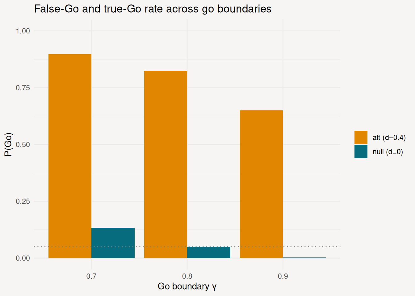
The choice of go boundary γ controls the tradeoff between false-Go rate (under the null, δ = 0) and true-Go rate (under the alternative, δ = 0.4). Stricter boundaries (higher γ) reduce false Go decisions at the cost of missing real effects. Since the posterior probability post_prob_delta does not depend on γ, we simulate both truths once and apply γ ∈ {0.7, 0.8, 0.9} in post-processing; two simulation runs, not six.
Collect posterior probabilities for null and alternative, then apply go boundaries
set.seed(77)
n_reps_oc <- 300

truths <- tibble::tibble(delta_true = c(0, 0.4))

post_by_truth <- purrr::pmap(truths, function(delta_true) {
  pop_oc <- list(
    placebo   = function(n) data.frame(id = 1:n, y = rnorm(n, 0,           sigma_known), readout_time = 1),
    treatment = local({ d <- delta_true
      function(n) data.frame(id = 1:n, y = rnorm(n, d, sigma_known), readout_time = 1)
    })
  )
  an_oc <- list(final = list(
    trigger  = enroll_trigger(1.0, sample_size),
    analysis = function(df, ct) {
      dat <- dplyr::filter(df, !is.na(enroll_time)) |>
        dplyr::mutate(arm = factor(arm, levels = c("placebo", "treatment")))
      pp <- RBesT::postmix(prior_placebo,   n = sum(dat$arm == "placebo"),   m = mean(dat$y[dat$arm == "placebo"]))
      pt <- RBesT::postmix(prior_treatment, n = sum(dat$arm == "treatment"), m = mean(dat$y[dat$arm == "treatment"]))
      data.frame(post_prob = RBesT::pmixdiff(pt, pp, delta, lower.tail = FALSE))
    }
  ))
  tr <- replicate_trial("oc", sample_size, arms, allocation,
                        enrollment_fn, dropout_fn, an_oc, pop_oc, n_reps_oc)
  invisible(run_trials(tr))
  collect_results(tr) |> dplyr::transmute(delta_true = delta_true, post_prob)
}) |> purrr::list_rbind()

# Apply each go boundary in post-processing
go_oc <- tidyr::expand_grid(go_boundary = c(0.7, 0.8, 0.9), delta_true = c(0, 0.4)) |>
  dplyr::rowwise() |>
  dplyr::mutate(
    scenario = if (delta_true == 0) "null (d=0)" else "alt (d=0.4)",
    go_prob  = mean(post_by_truth$post_prob[post_by_truth$delta_true == delta_true] >= go_boundary)
  ) |>
  dplyr::ungroup()
go_oc
#> # A tibble: 6 × 4
#>   go_boundary delta_true scenario    go_prob
#>         <dbl>      <dbl> <chr>         <dbl>
#> 1         0.7        0   null (d=0)  0.133
#> 2         0.7        0.4 alt (d=0.4) 0.897
#> 3         0.8        0   null (d=0)  0.05
#> 4         0.8        0.4 alt (d=0.4) 0.823
#> 5         0.9        0   null (d=0)  0.00333
#> 6 0.9 0.4 alt (d=0.4) 0.65ggplot(go_oc, aes(factor(go_boundary), go_prob, fill = scenario)) +
geom_col(position = "dodge") +
geom_hline(yintercept = 0.05, linetype = 3, colour = "grey50") +
coord_cartesian(ylim = c(0, 1)) +
scale_fill_manual(values = c("#e18600", "#076d7e")) +
labs(
x = "Go boundary \u03b3",
y = "P(Go)",
fill = NULL,
title = "False-Go and true-Go rate across go boundaries"
)
Next steps
- Example 5 - seamless Phase IIa/IIb design using BayesianMCPMod
- Conditions and Triggers - adding interim looks to a Bayesian design