library(rxsim)
library(ggplot2)Example 1: Two arm | Fixed design | Continuous
two-arm
fixed design
continuous
t-test
Generator API,
enroll_trigger, and single final t-test: the minimal complete rxsim workflow.
This example simulates a parallel-group trial evaluating a new treatment against placebo on a continuous primary endpoint (e.g., a biomarker score). 100 subjects are randomised 1:1; a two-sample t-test is run at full enrollment. This is the simplest complete rxsim workflow using the generator API (replicate_trial). For a side-by-side comparison see Two API Styles.
Unique focus: generator API, enroll_trigger, single final analysis.
Scenario
sample_size   <- 100
arms          <- c("pbo", "trt")
allocation    <- c(1, 1)
delta         <- 0.57             # true effect (SD units)
enrollment_fn <- function(n) c(1, rep(0, n - 1))  # all enroll at t = 1 (single look)
dropout_fn    <- function(n) rep(0, n)            # no dropout

scenario <- tidyr::expand_grid(
  sample_size = sample_size,
  allocation  = list(allocation),
  delta       = delta
)
tidyr::expand_grid() embeds design parameters into every result row, making results self-documenting across parameter sweeps.
Populations
population_generators <- list(
  pbo = function(n) data.frame(id = 1:n, value = rnorm(n),       readout_time = 1),
  trt = function(n) data.frame(id = 1:n, value = rnorm(n, delta), readout_time = 1)
)
readout_time = 1 means the endpoint is observed 1 time unit after enrollment. The treatment arm has a mean shift of delta SD units over placebo.
Conditions
enroll_trigger(1.0, sample_size) fires once all 100 subjects are enrolled. subset(!is.na(enroll_time)) removes subjects allocated but not yet arrived.
analysis_generators <- list(
  final = list(
    trigger  = enroll_trigger(1.0, sample_size),
    analysis = function(df, current_time) {
      enrolled <- subset(df, !is.na(enroll_time))
      tt <- t.test(value ~ arm, data = enrolled)
      data.frame(
        scenario,
        n_total  = nrow(enrolled),
        mean_pbo = mean(enrolled$value[enrolled$arm == "pbo"]),
        mean_trt = mean(enrolled$value[enrolled$arm == "trt"]),
        p_value  = unname(tt$p.value)
      )
    }
  )
)
Simulate
set.seed(1)
trials <- replicate_trial(
  trial_name            = "example_1",
  sample_size           = sample_size,
  arms                  = arms,
  allocation            = allocation,
  enrollment            = enrollment_fn,
  dropout               = dropout_fn,
  analysis_generators   = analysis_generators,
  population_generators = population_generators,
  n                     = 3
)run_trials(trials)replicate_results <- collect_results(trials)
replicate_results
#> replicate timepoint analysis sample_size allocation delta n_total mean_pbo
#> 1 1 1 final 100 1, 1 0.57 100 -0.05835028
#> 2 2 1 final 100 1, 1 0.57 100 0.10388173
#> 3 3 1 final 100 1, 1 0.57 100 -0.26638111
#> mean_trt p_value
#> 1 0.4473172 3.527785e-02
#> 2 0.5237190 3.373503e-02
#> 3 0.5979843 1.473874e-05p_value varies across replicates because each replicate draws independent random data and a fresh enrollment schedule.
Power curve
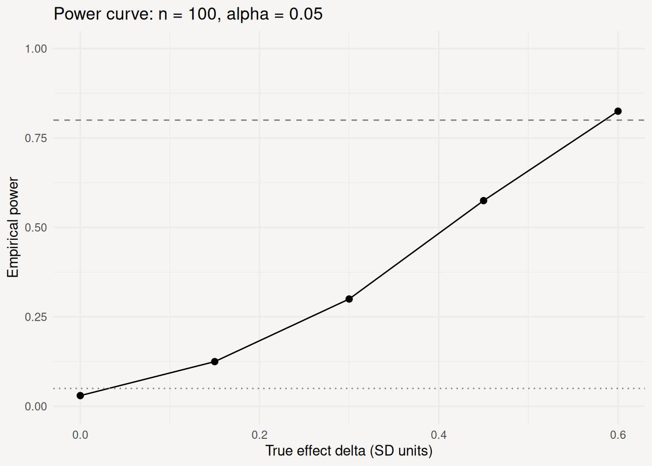
Running 500 replicates across a range of delta values reveals how power scales with effect size for n = 100 at alpha = 0.05.
Power curve sweep across effect sizes (delta = 0.00 to 0.60)
set.seed(42)
n_reps_pw <- 200

power_grid <- tibble::tibble(delta = seq(0, 0.6, by = 0.15))

power_df <- purrr::pmap(power_grid, function(delta) {
  pop_gens <- list(
    pbo = function(n) data.frame(id = 1:n, value = rnorm(n),        readout_time = 1),
    trt = function(n) data.frame(id = 1:n, value = rnorm(n, delta), readout_time = 1)
  )
  an_gens <- list(final = list(
    trigger  = enroll_trigger(1.0, sample_size),
    analysis = function(df, t) {
      e <- subset(df, !is.na(enroll_time))
      data.frame(p_value = t.test(value ~ arm, data = e)$p.value)
    }
  ))
  tr <- replicate_trial("pw", sample_size, arms, allocation,
                        enrollment_fn, dropout_fn, an_gens, pop_gens, n_reps_pw)
  invisible(run_trials(tr))
  data.frame(delta = delta, power = mean(collect_results(tr)$p_value < 0.05))
}) |> purrr::list_rbind()ggplot(power_df, aes(delta, power)) +
geom_line() +
geom_point(size = 2) +
geom_hline(yintercept = 0.80, linetype = 2, colour = "grey50") +
geom_hline(yintercept = 0.05, linetype = 3, colour = "grey50") +
coord_cartesian(ylim = c(0, 1)) +
labs(
x = "True effect delta (SD units)",
y = "Empirical power",
title = "Power curve: n = 100, alpha = 0.05"
)
Next steps
- Example 2 - adds a second endpoint
- Conditions and Triggers - in-depth guide to multi-look designs
- Population - endpoint data shapes for continuous, binary, and time-to-event outcomes