Example 3: Multi-arm | Fixed design | Single continuous endpoint | Dunnett test + MCP-Mod

Dose-response detection with Dunnett test and MCP-Mod across four active doses; DoseFinding::MCPMod.

# Core simulation framework (Timer, Population, Trial, deterministic_schedule, add_timepoints, ...)
library(rxsim)

# Analyses
library(multcomp)     # Dunnett
library(DoseFinding)  # MCP-Mod

# Helpers
library(dplyr)
library(ggplot2)
set.seed(4566)

Dose-finding trials aim to identify the dose-response relationship and establish an effective dose level. This example simulates a multi-arm fixed design across a placebo and four active doses, with the endpoint generated from an Emax dose-response model. At the final analysis, two methods are applied: a Dunnett test (comparing each active dose against placebo while controlling family-wise error rate) and MCP-Mod (a model-based contrast approach that selects the best-fitting dose-response shape from a candidate set).

Unique focus: multi-arm design, Emax dose-response data generation, Dunnett test vs MCP-Mod - comparing detection rates across effect sizes.

The simulation skeleton is the same as Example 1: define the scenario, create population generators, register conditions, and run replicate trials. This vignette focuses on what changes in a dose-finding setting.

Scenario

A multi-arm, fixed design (placebo + 4 active doses) with a single continuous endpoint. At the final analysis, we perform:

• Dunnett test: all active doses vs placebo using a normal-theory linear model.
• MCP-Mod: model-based multiple contrast test + model fitting on a candidate set of dose–response shapes.

The Emax model generates mean responses via E(d) = e0 + emax × d / (ed50 + d), where e0 = 0 (placebo baseline), emax = 1 (maximum achievable effect), and ed50 = 20 (dose at half-maximum effect). arm_names = paste0("d", doses) creates human-readable labels (d0, d5, d10, d20, d50) that propagate through trial data and analysis results. delta = 0.1 is the minimum effect size of clinical relevance used by MCP-Mod, and alpha = 0.05 controls the family-wise Type I error rate for both testing procedures.

# Dose levels (placebo + 4 actives)
doses <- c(0, 5, 10, 20, 50)

# Total N and allocation (balanced across arms)
sample_size <- 150
allocation  <- rep(1, length(doses))
arm_names   <- paste0("d", doses)  # e.g., d0, d5, ... used as arm labels

# Data-generating model: Emax with homoscedastic noise
e0    <- 0.0
emax  <- 1.0
ed50  <- 20.0
sigma <- 1.0

mean_fun <- function(d) e0 + emax * d / (ed50 + d)

# Operating characteristics
alpha <- 0.05
delta <- 0.1

scenario <- tidyr::expand_grid(
  sample_size = sample_size,
  allocation  = list(allocation),
  n_arms      = length(doses),
  alpha       = alpha,
  delta       = delta
)

enrollment_fn <- function(n) c(1, rep(0, n - 1))  # all enroll at t = 1 (single look)
dropout_fn    <- function(n) rep(0, n)            # no dropout

Populations

mk_pop_gen is a closure factory: it captures the dose value d and returns a generator function that, when called with n, draws n responses from N(E(d), sigma^2). Each arm’s generator stores dose as a numeric column because MCP-Mod requires actual dose values - not just arm labels - to fit dose-response models and evaluate contrasts at analysis time.

mk_pop_gen <- function(d) {
  function(n) {
    mu <- mean_fun(d)
    y  <- rnorm(n, mean = mu, sd = sigma)
    data.frame(
      id = seq_len(n),
      dose = d,
      y = y,
      readout_time = 1
    )
  }
}

population_generators <- lapply(seq_along(doses), function(i) {
  mk_pop_gen(doses[i])
})
names(population_generators) <- arm_names

Conditions

At the final time, run:

1. Dunnett test (active vs placebo) using multcomp::glht on lm(y ~ arm).

2. MCP-Mod using DoseFinding::MCPMod with a candidate model set (Mods).

The Dunnett test (multcomp::glht with mcp(arm = "Dunnett")) simultaneously compares each active dose against placebo while controlling the family-wise error rate at alpha. MCP-Mod is run with five candidate dose-response shapes; selModel = "aveAIC" selects the best model by AIC-weighted averaging, and Delta = delta sets the minimum effect size of clinical relevance for the contrast step. mct_min_p extracts the minimum p-value across all candidate model contrast tests - a small value indicates that at least one candidate model detects a dose-response signal.

# Candidate model set for MCP-Mod
mods <- Mods(
  linear     = NULL,
  emax       = 20,
  exponential= 50,
  sigEmax    = c(20, 3),
  quadratic  = -0.2,
  doses      = doses
)

analysis_generators <- list(
  final = list(
    trigger = enroll_trigger(1.0, sample_size),
    analysis = function(df, current_time){
      df_e <- df |>
        dplyr::filter(!is.na(enroll_time)) |>
        dplyr::mutate(
          arm  = factor(arm, levels = paste0("d", doses)),
          dose = as.numeric(dose)
        )

      # 1) Dunnett (active vs placebo)
      fit <- lm(y ~ arm, data = df_e)
      dun  <- multcomp::glht(fit, linfct = multcomp::mcp(arm = "Dunnett"))
      summ <- summary(dun)

      # 2) MCP-Mod (one-step)
      mm <- DoseFinding::MCPMod(
          dose   = df_e$dose,
          resp   = df_e$y,
          models = mods,
          type   = "normal",
          Delta  = delta,
          alpha  = alpha,
          selModel = "aveAIC"
      )

      mct_min_p <- min(attr(mm$MCTtest$tStat, "pVal"), na.rm = TRUE)

      data.frame(
        scenario,
        n_total      = nrow(df_e),
        dunn_min_p   = summ$test$pvalues |> as.numeric() |> min(),
        mcpmod_min_p = mct_min_p,
        stringsAsFactors = FALSE
      )
    }
  )
)

Simulate

set.seed(5)
trials <- replicate_trial(
  trial_name            = "multiarm_dunnett_mcpmod",
  sample_size           = sample_size,
  arms                  = arm_names,
  allocation            = allocation,
  enrollment            = enrollment_fn,
  dropout               = dropout_fn,
  analysis_generators   = analysis_generators,
  population_generators = population_generators,
  n                     = 3
)
run_trials(trials)

Results

collect_results() row-binds analysis outputs across all replicates and prepends replicate, timepoint, and analysis columns. dunn_min_p is the smallest Dunnett-adjusted p-value across the four active-dose comparisons - a value below alpha indicates that at least one dose significantly differs from placebo after multiplicity correction. mcpmod_min_p is the minimum MCP-Mod contrast test p-value across candidate models; MCP-Mod is generally more powerful when the true dose-response shape is well-captured by one of the candidate models.

replicate_results <- collect_results(trials)
replicate_results
#>   replicate timepoint analysis sample_size    allocation n_arms alpha delta
#> 1         1         1    final         150 1, 1, 1, 1, 1      5  0.05   0.1
#> 2         2         1    final         150 1, 1, 1, 1, 1      5  0.05   0.1
#> 3         3         1    final         150 1, 1, 1, 1, 1      5  0.05   0.1
#>   n_total   dunn_min_p mcpmod_min_p
#> 1     150 0.0002793752 8.152501e-05
#> 2     150 0.0030169849 2.794260e-05
#> 3     150 0.0048595026 2.505882e-04

Power curve

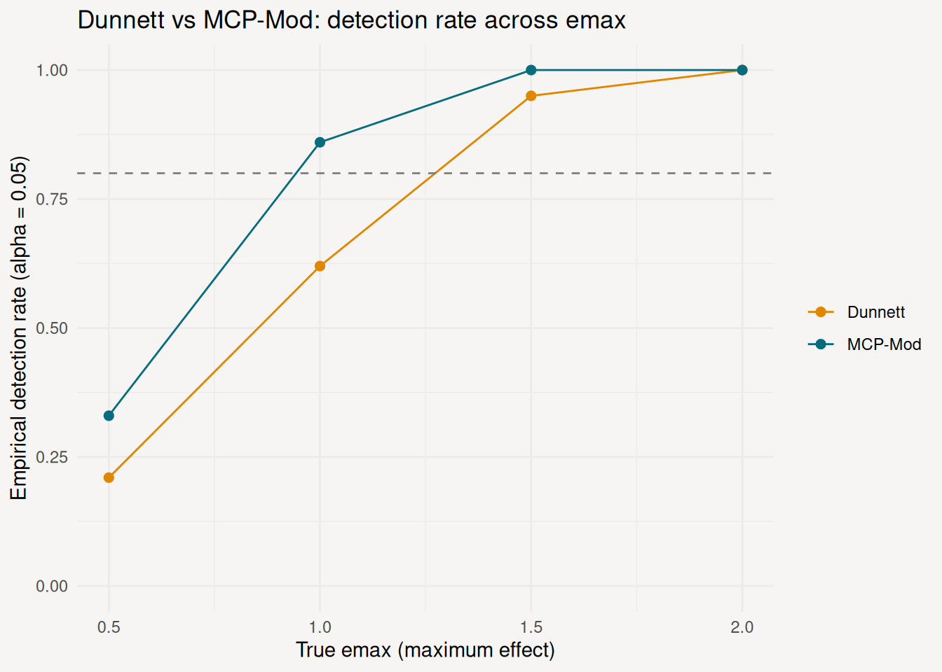
How does detection rate scale with the true maximum effect (emax)? We sweep emax over four values, keeping ed50 = 20 and n = 150 fixed, and compare the Dunnett and MCP-Mod rejection rates.

set.seed(55)
n_reps_pw <- 100

emax_grid <- tibble::tibble(emax = c(0.5, 1.0, 1.5, 2.0))

pw_df5 <- purrr::pmap(emax_grid, function(emax) {
  mf <- function(d) emax * d / (20 + d)
  pop_pw <- lapply(seq_along(doses), function(i) {
    d    <- doses[i]
    mu_d <- mf(d)
    function(n) data.frame(id = 1:n, dose = d, y = rnorm(n, mu_d, sigma), readout_time = 1)
  })
  names(pop_pw) <- arm_names

  an_pw <- list(final = list(
    trigger  = enroll_trigger(1.0, sample_size),
    analysis = function(df, ct) {
      df_e <- dplyr::filter(df, !is.na(enroll_time)) |>
        dplyr::mutate(
          arm  = factor(arm, levels = arm_names),
          dose = as.numeric(dose)
        )
      fit <- lm(y ~ arm, data = df_e)
      dun <- multcomp::glht(fit, linfct = multcomp::mcp(arm = "Dunnett"))
      mm  <- DoseFinding::MCPMod(
        dose = df_e$dose, resp = df_e$y,
        models = mods, type = "normal",
        Delta = delta, alpha = alpha, selModel = "aveAIC"
      )
      data.frame(
        dunn_sig   = as.integer(min(summary(dun)$test$pvalues) < alpha),
        mcpmod_sig = as.integer(min(attr(mm$MCTtest$tStat, "pVal"), na.rm = TRUE) < alpha)
      )
    }
  ))
  tr <- replicate_trial(
    "pw5", sample_size, arm_names, allocation,
    enrollment_fn, dropout_fn, an_pw, pop_pw, n_reps_pw
  )
  invisible(run_trials(tr))
  res <- collect_results(tr)
  data.frame(
    emax          = emax,
    power_dunnett = mean(res$dunn_sig),
    power_mcpmod  = mean(res$mcpmod_sig)
  )
}) |> purrr::list_rbind()

pw_long5 <- tidyr::pivot_longer(
  pw_df5,
  c(power_dunnett, power_mcpmod),
  names_to = "method", values_to = "power"
)
pw_long5$method <- factor(
  pw_long5$method,
  levels = c("power_dunnett", "power_mcpmod"),
  labels = c("Dunnett", "MCP-Mod")
)

ggplot(pw_long5, aes(emax, power, colour = method)) +
  geom_line() +
  geom_point(size = 2) +
  geom_hline(yintercept = 0.80, linetype = 2, colour = "grey50") +
  scale_colour_manual(values = c("#e18600", "#076d7e")) +
  coord_cartesian(ylim = c(0, 1)) +
  labs(
    x = "True emax (maximum effect)",
    y = "Empirical detection rate (alpha = 0.05)",
    title = "Dunnett vs MCP-Mod: detection rate across emax",
    colour = NULL
  )

Next steps

• Example 4 - Bayesian Go/No-Go with historical placebo borrowing
• Population - endpoint data setup for continuous, binary, and time-to-event outcomes