Binary Endpoints in Bayesian MCP-Mod

Show code

suppressPackageStartupMessages({
  library(BayesianMCPMod)
  library(RBesT)
  library(DoseFinding)
  library(dplyr)
})

set.seed(7015)

display_params_table <- function(named_list) {
  round_numeric <- function(x, digits = 3) if (is.numeric(x)) round(x, digits) else x
  tbl <- data.frame(
    Name  = names(named_list),
    Value = I(lapply(named_list, function(v) {
      if (inherits(v, "Date")) v <- as.character(v)
      if (!is.null(names(v))) paste0("{", paste(names(v), v, sep="=", collapse=", "), "}")
      else v
    }))
  )
  tbl$Value <- lapply(tbl$Value, round_numeric)
  knitr::kable(tbl)
}

Introduction

This vignette demonstrates the application of the BayesianMCPMod package for a binary endpoint. A more detailed introduction is provided for the setting of a continuous endpoint (analysis example vignette).

Binary endpoints require modeling on the logit scale. We will use the migraine dataset from the DoseFinding package as our working example, which contains response rates after migraine treatment. The prior (for the control group) will be based on historical trial data.

This package makes use of the future framework for parallel processing, which can be set up as follows:

future::plan(future::multisession)

Scale conventions used in this vignette

Scale conventions

Internally, BayesianMCPMod fits binary endpoints on the logit scale.
probability_scale = TRUE controls whether outputs (summaries, predictions, plots) are transformed back to probabilities.
delta for MED is interpreted on the probability scale when probability_scale = TRUE.

Calculation of a MAP Prior

In a first step, a meta analytic prior will be calculated. This prior is based on trials results for (Diener et al. 2011), (Ho et al. 2008) and (Hewitt et al. 2011). Here we assume the following historical results for the control group. Please note that only information from the control group will be integrated leading to an informative mixture prior for the control group, while for the active groups a non-informative prior will be specified.

Show code

study <- c("study 1", "study 2", "study 3")
n <- c(70,  115, 147) #sample size per study
r <- c(6,   16, 16) # responder per study

Our approach to establish a MAP prior is conducted in 3 steps. First the information from the historical trials is used to establish a beta mixture MAP prior (family=binomial).
In a next step this prior is robustified. Finally, since the BayesianMCPMod procedure for binary endpoints requires a prior on the logit scale, we translate this prior to this scale via sampling from the distribution, transitioning the individual results to the logit scale and approximating via fitting of normal mixtures of conjugate distributions. Please note that there would be various other options to establish a reasonable informative prior in this setting.

Show code

dose_levels <- c(0, 2.5, 5, 10, 20, 50, 100, 200)


#i) Establish MAP prior (beta mixture distribution)
set.seed(7015) # re-set seed only for this example; remove in your analysis script
map <- gMAP(
  cbind(r, n - r) ~ 1 |
    study,
  family = binomial,
  tau.dist = "HalfNormal",
  tau.prior = 0.5,
  beta.prior = (1 / sqrt(0.1 * 0.9)),
  warmup = 1000,
  iter = 10000,
  chains = 2,
  thin = 1
)
#> Assuming default prior location   for beta: 0
map
#> Generalized Meta Analytic Predictive Prior Analysis
#> 
#> Call:  gMAP(formula = cbind(r, n - r) ~ 1 | study, family = binomial, 
#>     tau.dist = "HalfNormal", tau.prior = 0.5, beta.prior = (1/sqrt(0.1 * 
#>         0.9)), iter = 10000, warmup = 1000, thin = 1, chains = 2)
#> 
#> Exchangeability tau strata: 1 
#> Prediction tau stratum    : 1 
#> Maximal Rhat              : 1 
#> 
#> Between-trial heterogeneity of tau prediction stratum
#>   mean     sd   2.5%    50%  97.5% 
#> 0.2710 0.2210 0.0106 0.2160 0.8290 
#> 
#> MAP Prior MCMC sample
#>   mean     sd   2.5%    50%  97.5% 
#> 0.1190 0.0494 0.0454 0.1130 0.2340
prior <- automixfit(map) #fits mixture distribution from MCMC samples from above
#ess(prior)
p <- summary(prior)[1]
#ii) Robustify prior
prior.rob <- RBesT::robustify(priormix = prior,
                              mean     = 0.5,
                              weight   = 0.4)

#ess(prior.rob)

#iii) Translate prior to logit scale (to approximate via normal mixture model)
r <- rmix(prior.rob, n = 1e4)
log.r <- RBesT::logit(r)
prior.ctr <- automixfit(log.r, type = "norm")
sigma(prior.ctr) <- sqrt(1 / (p * (1 - p)))
#ess(prior.ctr, sigma = sqrt(1/(p*(1-p))))
#Specification of reference scale (this follows the idea of [@Neuenschwander2016]).


#Specify a prior list
prior_trt <- RBesT::mixnorm(
  comp1 = c(
    w = 1,
    m = logit(summary(prior)[1]),
    n = 1
  ),
  sigma = sqrt(1 / (p * (1 - p))),
  param = "mn"
)

prior_list <- c(list(prior.ctr), rep(x     = list(prior_trt), times = length(dose_levels[-1])))

dose_names <- c("Ctr", paste0("DG_", seq_along(dose_levels[-1])))
names(prior_list) <- dose_names

Dose-Response Model Shapes

Candidate models are specified on the parameter scale using the {DoseFinding} package. We will create a Mods object, which will be used in the remainder of the vignette. Please note that the models are specified on the logit scale.

Show code

models <- Mods(
  linear = NULL,
  sigEmax = c(50, 3),
  quadratic = -1 / 250,
  logistic = c(110, 15),
  exponential = 80,
  emax = 10,
  doses = dose_levels,
  placEff = RBesT::logit(0.118),
  maxEff = RBesT::logit(0.3) - RBesT::logit(0.118)
)

plot(models)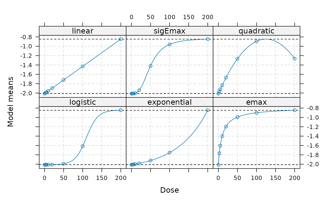

Trial Data

We will use the trial data from the migraine data set available in the DoseFinding package as our phase 2 trial data. We will apply a logistic regression (without any additional covariates) to get estimates on the logit scale.

Show code


data("migraine") #example data "migraine" from DoseFinding package

dosesFact <- as.factor(dose_levels)
N <- migraine$ntrt
RespRate <- migraine$painfree/N

##Execution of logistic regression and readout of parameters 
## (please note that estimates are automatically on logit scale)
logfit <- glm(RespRate ~ dosesFact - 1, family = binomial, weights = N)
muHat <- coef(logfit)
S <- vcov(logfit)

Posterior Calculation

In the first step of Bayesian MCPMod, the posterior is calculated by combining the prior information with the estimated results of the trial (Fleischer F 2022).

The summary of the posterior can be provided on the probability scale.

Show code

PostLogit<-getPosterior(prior_list,mu_hat=muHat,S_hat=S)

summary(PostLogit,probability_scale=TRUE)
#>           mean         sd       2.5%     50.0%     97.5%
#> Ctr  0.1071168 0.02127962 0.06930686 0.1058282 0.1520040
#> DG_1 0.1359001 0.06177459 0.04833967 0.1248126 0.2859179
#> DG_2 0.1222136 0.05057452 0.04865093 0.1137505 0.2436500
#> DG_3 0.2562256 0.05432101 0.16104931 0.2524449 0.3726678
#> DG_4 0.1943149 0.04961478 0.11121906 0.1895612 0.3041997
#> DG_5 0.2184915 0.05083942 0.13146633 0.2142515 0.3293963
#> DG_6 0.2401204 0.05496681 0.14521827 0.2358212 0.3591977
#> DG_7 0.3618200 0.06188555 0.24769337 0.3594987 0.4889697

Bayesian MCPMod Test Step

The testing step of Bayesian MCPMod is executed using a critical value on the probability scale and a pseudo-optimal contrast matrix.

A contrast matrix is generated based on the number of patients per dose group (see (Fleischer F 2022) for more details). Please note that here also other options would be possible (e.g. using weight based on the observed variability).

The critical value is calculated using (re-estimated) contrasts for frequentist MCPMod to ensure error control when using weakly-informative priors.

Show code


contr_mat_prior <- getContr(
  mods           = models,
  dose_levels    = dose_levels,
  dose_weights   = N)

set.seed(7015) # re-sets seed only for this example; remove in your analysis script
crit_pval <- getCritProb(
  mods           = models,
  dose_levels    = dose_levels,
  cov_new_trial   = S,
  alpha_crit_val = 0.05
)

The Bayesian MCP testing step is then executed:

Show code


BMCP_result <- performBayesianMCP(
  posterior_list = PostLogit,
  contr          = contr_mat_prior, 
  crit_prob_adj  = crit_pval)

Here as well it should be noted that this evaluation happens on the logit scale.

Summary information:

BMCP_result
#> Bayesian Multiple Comparison Procedure
#>   Significant:                   1 
#>   Critical Probability:          0.9790239 
#>   Maximum Posterior Probability: 0.99999 
#> Posterior Probabilities for Model Shapes
#>                        lin      sigE      quad       log       exp      emax
#>   Posterior Prob 0.9999900 0.9999338 0.9998325 0.9999509 0.9999644 0.9999885 
#>   Significant            1         1         1         1         1         1

The testing step is significant, indicating a non-flat dose-response shape. All models are significant.

Model Fitting and Visualization

In the model fitting step the posterior distribution is used as basis.

Both simplified and full fitting can be performed. Here we are focusing on the simplified fit. Furthermore we specify that the fit should be provided on the probability scale for easier interpretation of results.

The output of the fit includes information about the predicted effects for the included dose levels, the generalized AIC, and the corresponding weights.

Show code

##Perform modelling
model_fits <- getModelFits(
  models      = models,
  dose_levels = dose_levels,
  posterior   = PostLogit,
  simple      = TRUE,
  probability_scale = TRUE)

Plots of fitted dose-response models and an AIC-based average model including credible bands (orange shaded areas, default levels are 50% and 95%).:

#Default is on probability scale
plot(model_fits,cr_bands = TRUE)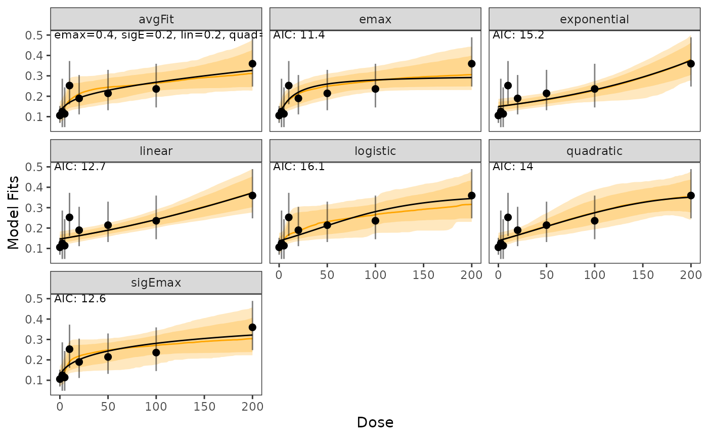

In case models should be shown on the logit scale this can be done in the following way:

plot(model_fits,probability_scale=FALSE)

Estimates (also for dose levels not included in the trial) can be shown via:

display_params_table(stats::predict(model_fits, doses = c(0, 2.5, 10,150, 200)))

	Name	Value
avgFit	avgFit	0.120, 0.140, 0.170, 0.300, 0.327
emax	emax	0.106, 0.133, 0.184, 0.288, 0.292
exponential	exponential	0.150, 0.151, 0.156, 0.294, 0.375
linear	linear	0.146, 0.148, 0.154, 0.303, 0.372
logistic	logistic	0.137, 0.141, 0.151, 0.323, 0.345
quadratic	quadratic	0.138, 0.141, 0.151, 0.325, 0.351
sigEmax	sigEmax	0.107, 0.143, 0.176, 0.305, 0.322

The bootstrap-based quantiles can also be directly calculated via the getBootstrapQuantiles() function and a sample from the model fits can be bootstrapped using getBootstrapSamples().

For this example, only 10 samples are bootstrapped for each model fit.

Show code

##Bootstrap quantiles
set.seed(7015) # re-sets seed only for this example; remove in your analysis script
bootstrap_quantiles <- getBootstrapQuantiles(
  model_fits = model_fits,
  quantiles  = c(0.025, 0.5, 0.975),
  doses      = dose_levels,
  n_samples  = 10)

Assessment of the Minimally Efficacious Dose

The Minimally Efficacious Dose (MED) per model shape can be assessed with the function getMED(). The effect needs to be specified on the probability scale.

##get MED

getMED(
  delta       = 0.16,
  model_fits  = model_fits,
  dose_levels = seq(min(dose_levels), max(dose_levels), by = 1))
#>             avgFit emax exponential linear logistic quadratic sigEmax
#> med_reached      1    1           1      1        1         1       1
#> med            118   59         161    153      117       121      78

Additional Note

Testing, modeling, and MED assessment can also be combined via performBayesianMCPMod():

Show code


BMCPMod_result <- performBayesianMCPMod(
  posterior_list = PostLogit,
  contr          = contr_mat_prior,
  crit_prob_adj  = crit_pval,
  simple         = TRUE,
  delta          = 0.16,
  probability_scale = TRUE
)

Diener, Hans-Christoph, Piero Barbanti, Carl Dahlöf, Uwe Reuter, Julia Habeck, and Jana Podhorna. 2011. “BI 44370 TA, an Oral CGRP Antagonist for the Treatment of Acute Migraine Attacks: Results from a Phase II Study.” Cephalalgia 31 (5): 573–84. https://doi.org/10.1177/0333102410388435.

Fleischer F, Deng Q, Bossert S. 2022. “Bayesian MCPMod.” Pharmaceutical Statistics 21 (3): 654–70.

Hewitt, D. J., V. Martin, R. B. Lipton, J. Brandes, P. Ceesay, R. Gottwald, E. Schaefer, C. Lines, and T. W. Ho. 2011. “Randomized Controlled Study of Telcagepant Plus Ibuprofen or Acetaminophen in Migraine.” Headache 51 (4): 533–43. https://doi.org/10.1111/j.1526-4610.2011.01860.x.

Ho, Tony W., Lauren K. Mannix, Xiaoyin Fan, Clara Assaid, Carol Furtek, Christopher J. Jones, Charles R. Lines, and Alan M. Rapoport. 2008. “Randomized Controlled Trial of an Oral CGRP Receptor Antagonist, MK-0974, in Acute Treatment of Migraine.” Neurology 70 (16): 1304–12. https://doi.org/10.1212/01.WNL.0000286940.29755.61.

2026-02-15

Introduction

Scale conventions used in this vignette

Calculation of a MAP Prior

Dose-Response Model Shapes

Trial Data

Posterior Calculation

Bayesian MCPMod Test Step

Model Fitting and Visualization

Assessment of the Minimally Efficacious Dose

Additional Note