Skip to contents
setup
#' Display Parameters Table
#'
#' This function generates a markdown table displaying the names and values of parameters
#' from a named list.
#'
#' @param named_list A named list where each name represents a parameter name and the list
#'   element represents the parameter value. Date values in the list are automatically
#'   converted to character strings for display purposes.
#'
#' @return Prints a markdown table with two columns: "Parameter Name" and "Parameter Values".
#'   The function does not return a value but displays the table directly to the output.
#'
#' @importFrom knitr kable
#' @examples
#' params <- list("Start Date" = as.Date("2020-01-01"),
#'                "End Date" = as.Date("2020-12-31"),
#'                "Threshold" = 10)
#' display_params_table(params)
#'
#' @export
display_params_table <- function(named_list) {
  display_table <- data.frame()
  value_names <- data.frame()
  for (i in 1:length(named_list)) {
    # dates will display as numeric by default, so convert to char first
    if (class(named_list[[i]]) == "Date") {
      named_list[[i]] = as.character(named_list[[i]])
    }
    if (!is.null(names(named_list[[i]]))) {
      value_names <- rbind(value_names, paste(names(named_list[[i]]), collapse = ', '))
    }
    values <- data.frame(I(list(named_list[[i]])))
    display_table <- rbind(display_table, values)
  }
  
  round_numeric <- function(x, digits = 3) {
    if (is.numeric(x)) {
      return(round(x, digits))
    } else {
      return(x)
    }
  }
  
  display_table[1] <- lapply(display_table[1], function(sublist) {
    lapply(sublist, round_numeric)
  })
  
  class(display_table[[1]]) <- "list"
  
  if (nrow(value_names) == 0) {
    knitr::kable(
      cbind(names(named_list), display_table),
      col.names = c("Name", "Value")
    )
  } else {
    knitr::kable(
      cbind(names(named_list), value_names, display_table),
      col.names = c("Name", "Value Labels", "Value")
    )
  }
}
# function to solve power results for tables (different max eff) BayesianMCPMod
# return(successrates models, average)
extract_success_rates <- function(results_list, models) {
  success_rates <- list()

  for (i in seq_along(results_list)) {
    success_rate <- c()
    for (model in models) {
      success_rate <- c(success_rate, attr(results_list[[i]][[model]]$BayesianMCP,"successRate"))
    }
    success_rates[[paste0("Bay_",  attr(results_list[[i]],"maxEff"))]] <- c(success_rate, attr(results_list[[i]], "avgSuccessRate"))
  }

  return(success_rates)
  }

# function to solve power results for tables (different nsample) BayesianMCPMod
#models <c-(min_scenario)
extract_success_rates_nsample <- function(results_list, models) {
  success_rates <- list()

  for (i in seq_along(results_list)) {
    success_rate <- c()
    for (model in models) {
      success_rate <- c(success_rate, attr(results_list[[i]][[model]]$BayesianMCP,"successRate"))
    }
    success_rates[[paste0("Bay_", i )]] <- c(success_rate,  attr(results_list[[i]],"avgSuccessRate"))
  }

  return(success_rates)
}

#input: result_list, models =
extract_success_rates_nsim <- function(results_list, models, n_sim) {
  success_rates <- list()
  for (model in models) {
    success_rate <- c()
    for (i in seq_along(n_sim)) {

      success_rate <- c(success_rate, attr(results_list[[i]][[model]]$BayesianMCP,"successRate"))
    }
    success_rates[[paste0("Bay_", model)]] <- c(success_rate)
  }

  return(success_rates)
}


print_result_Bay_max_eff <- function(results, scenario, variable) {

  result_table <- t(data.table(
    Bay_0.00 = results$`Bay_1e-04`,
    Bay_0.05 = results$Bay_0.05,
    Bay_0.1 = results$Bay_0.1,
    Bay_0.2 = results$Bay_0.2,
    Bay_0.3 = results$Bay_0.3,
    Bay_0.5 = results$Bay_0.5))

  result_table <- as.data.table(result_table)
  names(result_table) <- scenario
  #return(result_table)

  kable_result <- kable(cbind(variable, result_table))%>%
    kable_classic(full_width = TRUE)%>%
    add_header_above(c("Power results different expected effects " = length(scenario)+1), font_size = 15, bold = TRUE)%>%
    add_header_above(c("BayesianMCPMod " = length(scenario)+1), font_size = 15, bold = TRUE)

  list(result_table = result_table, kable_result = kable_result)
}


print_result_Bay_nsample <- function(results, scenario, variable) {

  result_table <- t(data.table(
    Bay_1 = results$Bay_1,
    Bay_2 = results$Bay_2,
    Bay_3 = results$Bay_3,
    Bay_4 = results$Bay_4))

  result_table <- as.data.table(result_table)
  names(result_table) <- scenario
  #return(result_table)

  kable_result <- kable(cbind(variable, result_table))%>%
    kable_classic(full_width = TRUE)%>%
    add_header_above(c("Success probability results different sample sizes " = length(scenario)+1), font_size = 15, bold = TRUE)%>%
    add_header_above(c("BayesianMCPMod " = length(scenario)+1), font_size = 15, bold = TRUE)

  list(result_table = result_table, kable_result = kable_result)
}

plot_power_deviation <- function(data, x, xlab){
  plot <- ggplot2::ggplot(data, aes(x = x, y = value, color = variable, group = variable))+
    geom_point()+
    geom_line() +
    scale_x_continuous(breaks = c(0, 100, 500, 1000, 2500, 5000, 10000),
    labels = c("", "100", "", "1000", "2500", "5000", "10000")) +
    geom_hline(aes(yintercept = 0), linetype = 2)+
    geom_hline(aes(yintercept = -0.05), linetype = 2, color = "darkgrey")+
    geom_hline(aes(yintercept = 0.05), linetype = 2, color = "darkgrey")+
    geom_hline(aes(yintercept = -0.1), linetype = 2, color = "darkgrey")+
    geom_hline(aes(yintercept = 0.1), linetype = 2, color = "darkgrey")+
    scale_color_manual(name = "assumed true model", values = c("linear" = "red", "exponential" = "blue", "emax" = "darkgreen", "logistic" = "orange", "sigemax" = "purple", "beta" = "deepskyblue", "quadratic" = "deeppink"))+
    labs(x = xlab, y = "power deviation")+
    ylim(-0.15, 0.15)+        
    theme_classic()
  return(plot)
}


# parallel----------------------------------------------
chunkVector <- function (x, n_chunks) {
  if (n_chunks <= 1) {
    chunk_list <- list(x)
  } else {
    chunk_list <- unname(split(x, cut(seq_along(x), n_chunks, labels = FALSE)))
  }
  return(chunk_list)
}


library(BayesianMCPMod)
library(RBesT)
library(clinDR)
library(dplyr)
library(tibble)
library(reactable)
library(DoseFinding)
library(MCPModPack)
library(kableExtra)
library(data.table)
library(doFuture)
library(doRNG)

registerDoFuture()
plan(multisession)


set.seed(7015)

1 Introduction

This vignette demonstrates the application of the {BayesianMCPMod} package for sample size calculations and the comparison with the {MCPModPack} package. As for other bayesian approaches BMCPMod is set up in a way that it mimics the results (and operating characteristics) of the frequentist MCPMod for non-informative priors. This characteristic is illustrated in the following sections focusing on the trial planning.

In order to compare BayesianMCPMod and MCPModPack success probabilities the following dose-finding scenario is considered.

  • four dose levels plus placebo (0 mg, 1 mg, 2 mg, 4 mg, 8 mg)

  • total sample size of N = 200

  • equal allocation ratio for each dose group (i.e. 40 per group)

  • standard deviation of 0.4 for every dose group

  • alpha level of 5%

Building on this scenario the following varying effects are used:

  • expected effect for maximum dose of (0.0001,0.05, 0.1, 0.2, 0.3, 0.5)

Technical note: The value of 0.0001 was chosen instead of 0 due to technical reasons. This case should mimic the null scenario (where we expect a success probability close to the alpha level). For each of these simulation cases, 10000 simulation runs are performed. Given the number of simulations, and using basic mathematical approximations (like the law of large numbers) the difference in success probabilities should be in the range of 1-3%.

setup
#######  General assumptions  #########
# simulations
n_sim <- 1000 #to be upscaled to 10000

# define input parameters
doses.sim <- c(0,1,2,4,8)   # dose levels
max.dose <- max(doses.sim) # specify max dose possibly available
plc.guess <-  0 # expected placebo effect
Nsample <-c(40,40,40,40,40) #,36*c(1,1,1,1)) #list(20*c(2,1,1,2),30*c(1,1,1,1), 24*c(2,1,1,2),36*c(1,1,1,1))
expectedEffect_fix <- 0.2  #c(0.05,0.1,0.2,0.3,0.5)
expectedEffect <- c(0.0001,0.05,0.1,0.2,0.3,0.5)
sd.sim <- c(0.4)


# define model functions  
emax.g <- guesst(d = doses.sim[2], p = 0.6, "emax") 
exp.g <- guesst(d=doses.sim[2],p=0.05,model="exponential", Maxd=max.dose)
logit.g <- guesst(d=c(doses.sim[2],doses.sim[3]),p=c(0.1,0.9),"logistic",Maxd=max.dose) 
sigEmax.g <- guesst(d=c(doses.sim[2],doses.sim[3]),p=c(0.15,0.75), model = "sigEmax") 
#quad.g <- guesst(d=doses.sim[2],p=0.35,model="quadratic")
#beta.g <- guesst(d=doses.sim[2],p=0.2,model="betaMod", dMax=5.5, scal=9.6, Maxd=max.dose)

### define models to be tested in MCPMod
models <- Mods(linear=NULL, 
               emax = emax.g,
               exponential = exp.g,
               logistic=logit.g,
               sigEmax = sigEmax.g,
               #quadratic = quad.g,
               #betaMod = beta.g,
               doses = doses.sim,
               placEff = plc.guess, 
               maxEff = expectedEffect_fix,
               direction = "increasing",
               addArgs = list(scal=9.6) 
)

alpha <- 0.05

# display_params_table(models)


# kable(t(as.data.table(cbind(doses.sim, Nsample))))%>%
#     kable_classic(full_width = TRUE)%>%
#     add_header_above(c( "Doses" = 6), font_size = 15, bold = TRUE)
# 
# 
# kable(t(data.table(placebo_guess = plc.guess,
#                  sd = sd.sim[1],
#                  alpha = alpha )))%>%
#     kable_classic(full_width = TRUE)

1.1 Scenarios

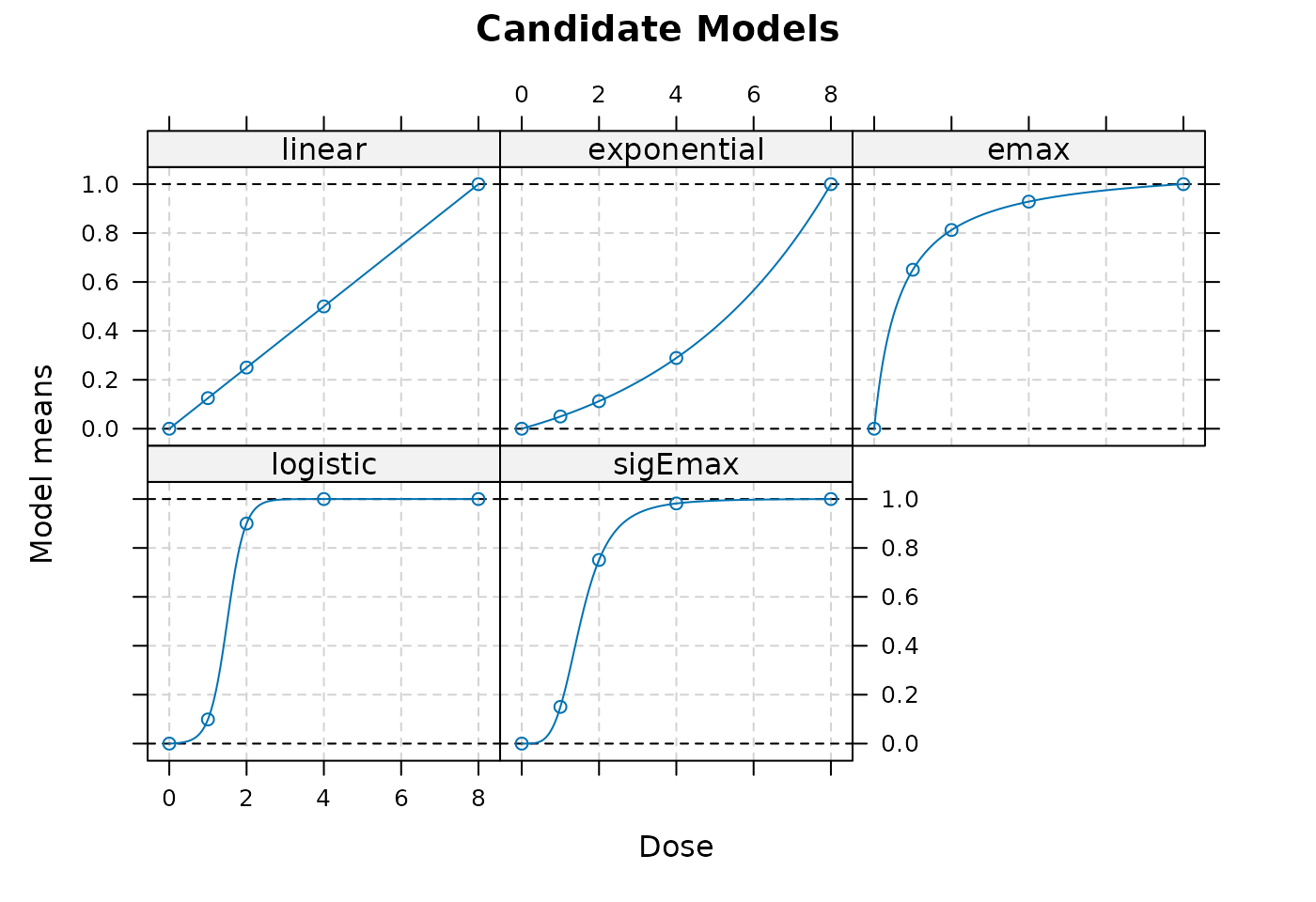
In the following the candidate models are specified and plotted.

setup
#Specification of considered models for different scenarios for BayesianMCPMod

monotonic_scenario <- c("linear", "exponential", "emax", "logistic", "sigEmax")

monotonic_models <- Mods(linear=NULL, 
               exponential = exp.g,
               emax = emax.g,
               logistic=logit.g,
               sigEmax = sigEmax.g,
               doses = doses.sim,
               placEff = plc.guess, 
               maxEff = expectedEffect_fix,
               direction = "increasing"
)
plot(monotonic_models, main = "monotonic Scenario")

2 MCPModPack

setup
#Specification of considered models for MCPModPack
monotonic_modelsPack = list(linear = NA,
              exponential = 4.447149,
              emax = 0.6666667,
              logistic = c(1.5, 0.2275598),
              sigEmax =  c(1.528629, 4.087463))

The following simulations will be conducted utilizing the MCPModPack package (with varying expected effect for maximum dose and sample sizes).

2.1 Monotonic scenario

2.1.1 varying expected effect for maximum dose

setup
# assumed dose - response models
sim_models_monotonic_linear = list(linear = NA,
                  max_effect =expectedEffect ,
                  sd = rep(sd.sim, length(doses.sim)),
                  placebo_effect = plc.guess)

sim_models_monotonic_exp = list( exponential = 4.447149,
                  max_effect = expectedEffect,
                  sd = rep(sd.sim, length(doses.sim)),
                  placebo_effect = plc.guess)

sim_models_monotonic_logistic = list(logistic = c(1.5, 0.2275598),
                  max_effect = expectedEffect,
                  sd = rep(sd.sim, length(doses.sim)),
                  placebo_effect = plc.guess)

sim_models_monotonic_sigemax= list(sigemax =  c(1.528629, 4.087463),
                  max_effect = expectedEffect,
                  sd = rep(sd.sim, length(doses.sim)),
                  placebo_effect = plc.guess)

sim_models_monotonic_emax= list(emax = 0.6666667,
                  max_effect = expectedEffect,
                  sd = rep(sd.sim, length(doses.sim)),
                  placebo_effect = plc.guess)

# Simulation parameters
sim_parameters = list(n = Nsample, 
                      doses = doses.sim,
                      dropout_rate = 0.0, 
                      go_threshold = 0.1, 
                      nsims = n_sim)

# Initialize list to store results
results_list_monotonic <- list()

list_models <- list(sim_models_monotonic_linear, sim_models_monotonic_exp, sim_models_monotonic_emax, sim_models_monotonic_logistic, sim_models_monotonic_sigemax)
chunks <- chunkVector(seq_along(list_models), getDoParWorkers())

func_sim <- function(models ,sim_models, sim_parameters){

sim_result = MCPModSimulation(endpoint_type = "Normal", 
                                 models = models, 
                                 alpha = alpha, 
                                 direction = "increasing", 
                                 model_selection = "aveAIC", 
                                 Delta = 0.1,
                                 sim_models = sim_models,
                                 sim_parameters = sim_parameters)
}


results_list_monotonic <- foreach(k = chunks, .combine = c) %dorng% {
  
  lapply(k, function (i) {
    
    func_sim(monotonic_modelsPack, list_models[[i]], sim_parameters) 
    
  })
  
}
  

results_monotonic_MCP <- data.table(
  max_eff = expectedEffect,
  linear = c(results_list_monotonic[[1]]$sim_results$power),
  exp = c(results_list_monotonic[[2]]$sim_results$power),
  emax = c(results_list_monotonic[[3]]$sim_results$power),
  logistic = c(results_list_monotonic[[4]]$sim_results$power),
  sigEmax = c(results_list_monotonic[[5]]$sim_results$power),
  Average = c((sum(results_list_monotonic[[1]]$sim_results$power[1], results_list_monotonic[[2]]$sim_results$power[1], results_list_monotonic[[3]]$sim_results$power[1], results_list_monotonic[[4]]$sim_results$power[1], results_list_monotonic[[5]]$sim_results$power[1])/5),
  (sum(results_list_monotonic[[1]]$sim_results$power[2], results_list_monotonic[[2]]$sim_results$power[2], results_list_monotonic[[3]]$sim_results$power[2], results_list_monotonic[[4]]$sim_results$power[2], results_list_monotonic[[5]]$sim_results$power[2])/5),
              (sum(results_list_monotonic[[1]]$sim_results$power[3], results_list_monotonic[[2]]$sim_results$power[3], results_list_monotonic[[3]]$sim_results$power[3], results_list_monotonic[[4]]$sim_results$power[3], results_list_monotonic[[5]]$sim_results$power[3])/5),
(sum(results_list_monotonic[[1]]$sim_results$power[4], results_list_monotonic[[2]]$sim_results$power[4], results_list_monotonic[[3]]$sim_results$power[4], results_list_monotonic[[4]]$sim_results$power[4], results_list_monotonic[[5]]$sim_results$power[4])/5),
(sum(results_list_monotonic[[1]]$sim_results$power[5], results_list_monotonic[[2]]$sim_results$power[5], results_list_monotonic[[3]]$sim_results$power[5], results_list_monotonic[[4]]$sim_results$power[5], results_list_monotonic[[5]]$sim_results$power[5])/5))
)

#kable(results_monotonic_MCP)%>%
 # kable_classic(full_width = TRUE)%>%
  #  add_header_above(c("Power results different expected effects " = 7), font_size = 15, bold = TRUE)%>%
  #  add_header_above(c("Monotonic scenario " = 7), font_size = 15, bold = TRUE)

3 BayesianMCPMod

Following simulations will be conducted utilizing the ‘BayesianMCPMod’ package using the same scenarios as for the frequentist evaluations.

4 Prior Specification

In a first step a non-informative prior is specified.

setup
uninf_prior_list <- list(
                   Ctrl = RBesT::mixnorm(comp1 = c(w = 1, m = 0, n = 1), sigma = sd.sim, param = "mn"),
                   DG_1 = RBesT::mixnorm(comp1 = c(w = 1, m = 0, n = 1), sigma = sd.sim, param = "mn"),
                   DG_2 = RBesT::mixnorm(comp1 = c(w = 1, m = 0, n = 1), sigma = sd.sim, param = "mn"),
                   DG_3 = RBesT::mixnorm(comp1 = c(w = 1, m = 0, n = 1), sigma = sd.sim, param = "mn"),
                   DG_4 = RBesT::mixnorm(comp1 = c(w = 1, m = 0, n = 1), sigma = sd.sim, param = "mn")
                   
)

To calculate success probabilities for the different assumed dose-response models and the specified trial design we will apply the assessDesign function.

4.1 Monotonic scenario

4.1.1 varying expected effect for maximum dose

setup
results_list_Bay_monotonic <- list()


list_max_eff <- as.list(c(0.0001,0.05,0.1,0.2,0.3,0.5))
chunks <- chunkVector(seq_along(list_max_eff), getDoParWorkers())


results_list_Bay_monotonic <- foreach(k = chunks, .combine = c) %dorng% {
  
  lapply(k, function (i) {
    
    monotonic_models <- Mods(linear=NULL, 
                         exponential = exp.g,
                         emax = emax.g,
                         logistic=logit.g,
                         sigEmax = sigEmax.g,
                         doses = doses.sim,
                         placEff = plc.guess, 
                         maxEff = list_max_eff[[i]],
                         direction = "increasing")
       
  # optimal contrasts
  contM <- getContr(mods = monotonic_models, 
                    dose_levels = doses.sim, 
                    prior_list = uninf_prior_list, 
                    dose_weights = c(1,1,1,1,1))
  
  # perform Simulations
  success_probabilities_monotonic <- assessDesign(
    n_patients  = Nsample,
    mods        = monotonic_models,
    prior_list  = uninf_prior_list,
    sd          = sd.sim,
    n_sim       = n_sim,
    alpha_crit_val = alpha, 
    contr = contM)


  })
  
}
  

##power results in vector for tables
results_monotonic_Bay <- extract_success_rates(results_list_Bay_monotonic, monotonic_scenario)


monotonic_Bay <- print_result_Bay_max_eff(results_monotonic_Bay, c(monotonic_scenario, "average"), round(expectedEffect,3))
  

#monotonic_Bay$kable_result

5 Comparison

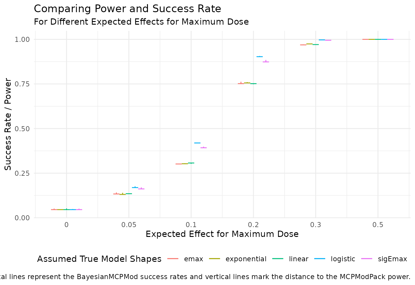
In the following, the comparisons between the success probabilities (i.e.power values for frequentist set-up) of various scenarios and different parameters are visualized.

The following plots show the difference between the results from MCPModPack and BayesianMCPMod. The results of MCPModPack are shown as a line and the difference to the result with BayesianMCPMod is presented as a bar. The results for the different assumed true dose-response models (that were the basis for simulating the data) are shown in different colours.

5.1 varying expected effect for maximum dose

5.1.1 monotonic scenario

setup
#table with results
kable(results_monotonic_MCP)%>%
  kable_classic(full_width = TRUE)%>%
    add_header_above(c("Power results different expected effects " = 7), font_size = 15, bold = TRUE)%>%
    add_header_above(c("MCPModPack " = 7), font_size = 15, bold = TRUE)
MCPModPack
Power results different expected effects
max_eff linear exp emax logistic sigEmax Average
1e-04 0.059 0.049 0.050 0.049 0.056 0.0526
5e-02 0.144 0.143 0.134 0.158 0.161 0.1480
1e-01 0.299 0.292 0.291 0.422 0.418 0.3444
2e-01 0.768 0.762 0.755 0.902 0.894 0.8162
3e-01 0.970 0.972 0.971 0.999 0.994 0.9812
5e-01 1.000 1.000 1.000 1.000 1.000 0.0526
setup
monotonic_Bay$kable_result
BayesianMCPMod
Power results different expected effects
variable linear exponential emax logistic sigEmax average
0.00 0.040 0.040 0.040 0.040 0.040 0.0400
0.05 0.141 0.129 0.138 0.179 0.172 0.1518
0.10 0.302 0.291 0.292 0.402 0.380 0.3334
0.20 0.752 0.749 0.740 0.889 0.844 0.7948
0.30 0.965 0.974 0.971 0.997 0.995 0.9804
0.50 1.000 1.000 1.000 1.000 1.000 1.0000
setup
data_plot_eff_monotonic <- data.frame(
  max_eff = expectedEffect,
  max_eff_num = c(1, 2, 3, 4, 5,6),
  start_linear =  results_monotonic_MCP$linear,
  end_linear =  monotonic_Bay$result_table$linear,
  start_exp = results_monotonic_MCP$exp,
  end_exp =  monotonic_Bay$result_table$exponential,
  start_emax = results_monotonic_MCP$emax,
  end_emax =   monotonic_Bay$result_table$emax,
  start_logistic = results_monotonic_MCP$logistic,
  end_logistic =  monotonic_Bay$result_table$logistic,
  start_sigemax = results_monotonic_MCP$sigEmax,
  end_sigemax =  monotonic_Bay$result_table$sigEmax
)


# Create the plot
ggplot(data = data_plot_eff_monotonic, aes(x = max_eff_num)) +
  geom_segment(aes(x = max_eff_num - 0.4, xend = max_eff_num - 0.4, y = start_linear, yend = end_linear, color = "linear", size = "BayesianMCPMod")) +
  geom_segment(aes(x = max_eff_num - 0.45, xend = max_eff_num - 0.35 , y = start_linear, yend = start_linear, color = "linear", size = "MCPModPack")) +
  geom_segment(aes(x = max_eff_num - 0.2, xend = max_eff_num - 0.2 , y = start_exp, yend = end_exp, color = "exponential", size = "BayesianMCPMod")) +
  geom_segment(aes(x = max_eff_num- 0.25, xend = max_eff_num - 0.15, y = start_exp, yend = start_exp, color = "exponential", size = "MCPModPack")) +
  geom_segment(aes(x = max_eff_num, xend = max_eff_num, y = start_emax, yend = end_emax, color = "emax", size = "BayesianMCPMod")) +
  geom_segment(aes(x = max_eff_num - 0.05, xend = max_eff_num + 0.05, y = start_emax, yend = start_emax, color = "emax", size = "MCPModPack")) +
  geom_segment(aes(x = max_eff_num + 0.2, xend = max_eff_num + 0.2, y = start_logistic, yend = end_logistic, color = "logistic", size = "BayesianMCPMod")) +
  geom_segment(aes(x = max_eff_num + 0.15, xend = max_eff_num + 0.25, y = start_logistic, yend = start_logistic, color = "logistic", size = "MCPModPack")) +
  geom_segment(aes(x = max_eff_num + 0.4, xend = max_eff_num + 0.4, y = start_sigemax, yend = end_sigemax, color = "sigemax", size = "BayesianMCPMod")) +
  geom_segment(aes(x = max_eff_num + 0.35, xend = max_eff_num + 0.45, y = start_sigemax, yend = start_sigemax, color = "sigemax", size = "MCPModPack")) +
  scale_x_continuous(breaks = data_plot_eff_monotonic$max_eff_num, labels = data_plot_eff_monotonic$max_eff) +
  scale_color_manual(name = "Assumed true model", values = c("linear" = "red", "exponential" = "blue", "emax" = "darkgreen", "logistic" = "orange", "sigemax" = "purple", "beta" = "deepskyblue", "quadratic" = "deeppink"))+
  scale_size_manual( name = "Package", values = c("MCPModPack" = 0.5, "BayesianMCPMod" = 2))+
  theme_minimal() +
  ylab("Power") +
  xlab("expected effect for maximum dose")+
  ggtitle("Power values different expected effect for maximum dose")+
  geom_vline(xintercept = data_plot_eff_monotonic$max_eff_num + 0.5, linetype="dashed", color = "black") +
  theme(legend.position = "bottom") +
  guides(color = guide_legend(nrow= 2 , byrow= TRUE ), size = guide_legend(nrow= 2 , byrow= TRUE )) 

As expected operating characteristics for BayesianMCPMod with non-informative prior match with operating characteristics for frequentist MCPMod.

5.2 convergence of power values

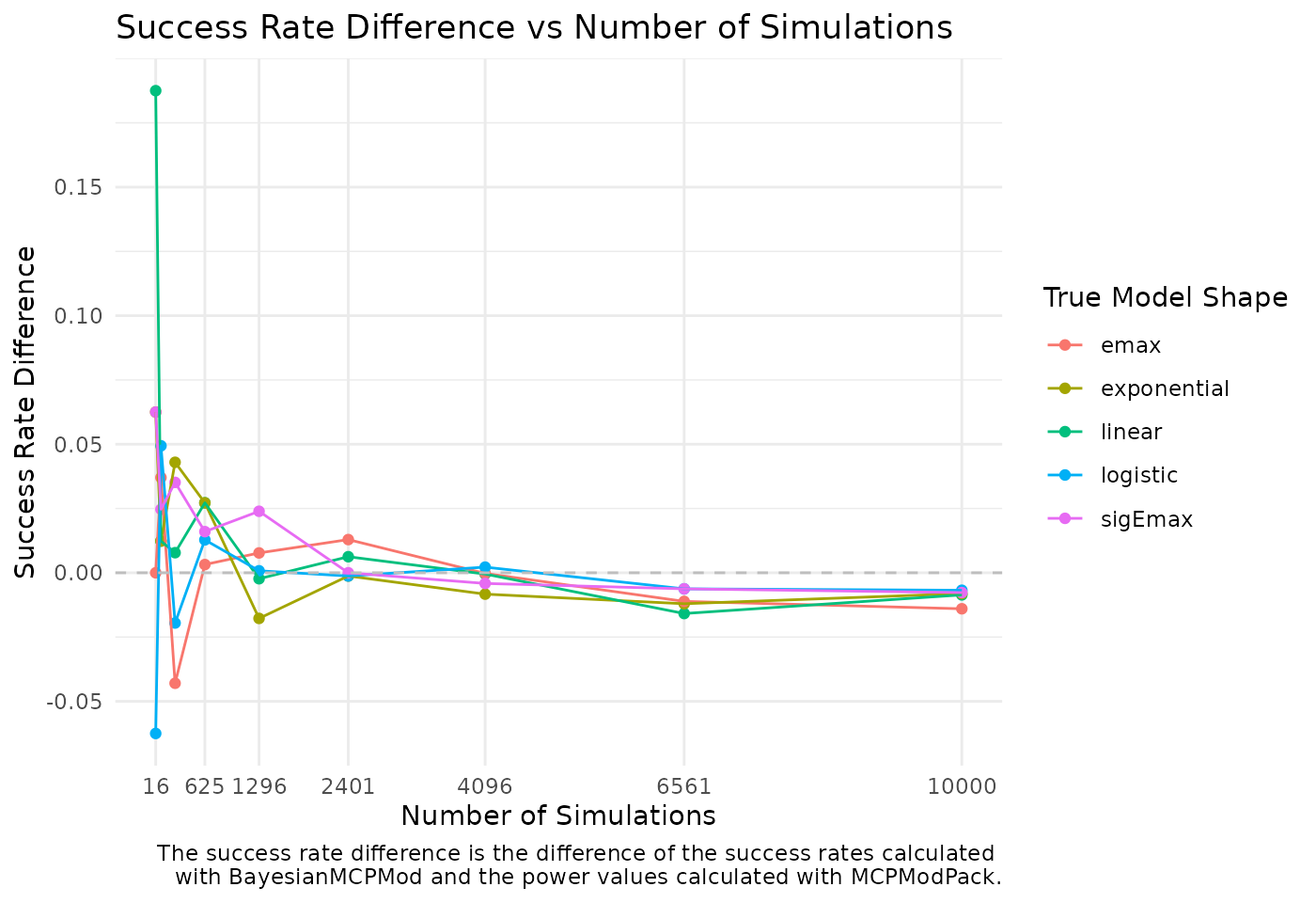
In the following simulations, we examine the convergence of power values for an increasing number of simulations. We are considering the following number of simulations: 100, 500, 1000, 2500, 5000, 10000.

5.2.1 monotonic BayesianMCPMod

setup
n_sim_values_list <- as.list(c(10, 50, 100, 250, 500, 1000)) #as.list(c(100, 500, 1000, 2500, 5000, 10000))
n_sim_values <- c(10, 50, 100, 250, 500, 1000) #c(100, 500, 1000, 2500, 5000, 10000)

# Initialize a list to store the results
 results_list_nsim_Bay_monotonic <- list()
 
monotonic_models <- Mods(linear=NULL,
                         exponential = exp.g,
                         emax = emax.g,
                         logistic=logit.g,
                         sigEmax = sigEmax.g,
                         doses = doses.sim,
                         placEff = plc.guess,
                         maxEff = expectedEffect_fix,
                         direction = "increasing")

#optimal contrasts
contM <- getContr(mods = monotonic_models,
                  dose_levels = doses.sim,
                  prior_list = uninf_prior_list,
                  dose_weights = c(1,1,1,1,1))

n_sim_values_list <- as.list(c(10, 50, 100, 250, 500, 1000)) #as.list(c(100, 500, 1000, 2500, 5000, 10000))

chunks <- chunkVector(seq_along(n_sim_values_list), getDoParWorkers())


results_list_nsim_Bay_monotonic <- foreach(k = chunks, .combine = c, .export = c(as.character(monotonic_models), as.character(contM))) %dorng% {

  lapply(k, function (i) {


 # Simulation step
  success_probabilities_monotonic <- assessDesign(
    n_patients  = Nsample,
    mods        = monotonic_models,
    prior_list  = uninf_prior_list,
    sd          = sd.sim,
    n_sim       = n_sim_values_list[[i]],
    alpha_crit_val = alpha,
    contr = contM)

  })

}


results_nsim_Bay_monotonic <- extract_success_rates_nsim(results_list_nsim_Bay_monotonic, monotonic_scenario, n_sim_values)

5.2.2 monotonic MCPModPack

setup
sim_models_monotonic_linear$max_effect <- expectedEffect_fix
sim_models_monotonic_exp$max_effect <- expectedEffect_fix
sim_models_monotonic_emax$max_effect <- expectedEffect_fix
sim_models_monotonic_logistic$max_effect <- expectedEffect_fix
sim_models_monotonic_sigemax$max_effect <- expectedEffect_fix

list_models <- list(sim_models_monotonic_linear, sim_models_monotonic_linear, sim_models_monotonic_linear, sim_models_monotonic_linear, sim_models_monotonic_linear, sim_models_monotonic_linear, 
                    sim_models_monotonic_exp, sim_models_monotonic_exp, sim_models_monotonic_exp, sim_models_monotonic_exp, sim_models_monotonic_exp, sim_models_monotonic_exp, 
                    sim_models_monotonic_emax, sim_models_monotonic_emax, sim_models_monotonic_emax, sim_models_monotonic_emax, sim_models_monotonic_emax, sim_models_monotonic_emax,
                    sim_models_monotonic_logistic, sim_models_monotonic_logistic, sim_models_monotonic_logistic, sim_models_monotonic_logistic, sim_models_monotonic_logistic, sim_models_monotonic_logistic,
                    sim_models_monotonic_sigemax, sim_models_monotonic_sigemax, sim_models_monotonic_sigemax, sim_models_monotonic_sigemax, sim_models_monotonic_sigemax, sim_models_monotonic_sigemax
                    )
n_sim_values_list <- as.list(c(10, 50, 100, 250, 500, 1000,
                               10, 50, 100, 250, 500, 1000,
                               10, 50, 100, 250, 500, 1000,
                               10, 50, 100, 250, 500, 1000,
                               10, 50, 100, 250, 500, 1000))
  
  #as.list(c(100, 500, 1000, 2500, 5000, 10000,
              #                 100, 500, 1000, 2500, 5000, 10000,
                 #              100, 500, 1000, 2500, 5000, 10000,
                  #             100, 500, 1000, 2500, 5000, 10000,
                    #           100, 500, 1000, 2500, 5000, 10000))

chunks <- chunkVector(seq_along(list_models), getDoParWorkers())

results_list_nsim_MCP_monotonic <- foreach(k = chunks, .combine = c, .export = c(as.character(monotonic_modelsPack)))  %dorng% {
  
  lapply(k, function (i) {
    # Simulation parameters
  sim_parameters = list(n = Nsample,
                      doses = doses.sim,
                      dropout_rate = 0.0,
                      go_threshold = 0.1,
                      nsims = n_sim_values_list[[i]])
    
    func_sim(monotonic_modelsPack, list_models[[i]], sim_parameters) 
    
  })
  
}

5.3 Results

The following plots show the result of the convergence test of the power values for an increasing number of simulations. The difference between the success probabilities of the frequency and Bayesian simulations is shown.

5.3.1 monotonic scenario

setup
#safe results in data.table for plot
results_nsim_monotonic <- data.table(
  MCP_linear = c(results_list_nsim_MCP_monotonic[[1]]$sim_results$power, results_list_nsim_MCP_monotonic[[2]]$sim_results$power, results_list_nsim_MCP_monotonic[[3]]$sim_results$power, results_list_nsim_MCP_monotonic[[4]]$sim_results$power, results_list_nsim_MCP_monotonic[[5]]$sim_results$power, results_list_nsim_MCP_monotonic[[6]]$sim_results$power),
  MCP_exp = c(results_list_nsim_MCP_monotonic[[7]]$sim_results$power, results_list_nsim_MCP_monotonic[[8]]$sim_results$power, results_list_nsim_MCP_monotonic[[9]]$sim_results$power, results_list_nsim_MCP_monotonic[[10]]$sim_results$power, results_list_nsim_MCP_monotonic[[11]]$sim_results$power, results_list_nsim_MCP_monotonic[[12]]$sim_results$power),
  MCP_emax = c(results_list_nsim_MCP_monotonic[[13]]$sim_results$power, results_list_nsim_MCP_monotonic[[14]]$sim_results$power, results_list_nsim_MCP_monotonic[[15]]$sim_results$power, results_list_nsim_MCP_monotonic[[16]]$sim_results$power, results_list_nsim_MCP_monotonic[[17]]$sim_results$power, results_list_nsim_MCP_monotonic[[18]]$sim_results$power),
  MCP_logistic = c(results_list_nsim_MCP_monotonic[[19]]$sim_results$power, results_list_nsim_MCP_monotonic[[20]]$sim_results$power, results_list_nsim_MCP_monotonic[[21]]$sim_results$power, results_list_nsim_MCP_monotonic[[22]]$sim_results$power, results_list_nsim_MCP_monotonic[[23]]$sim_results$power, results_list_nsim_MCP_monotonic[[24]]$sim_results$power),
  MCP_sigemax = c(results_list_nsim_MCP_monotonic[[25]]$sim_results$power, results_list_nsim_MCP_monotonic[[26]]$sim_results$power, results_list_nsim_MCP_monotonic[[27]]$sim_results$power, results_list_nsim_MCP_monotonic[[28]]$sim_results$power, results_list_nsim_MCP_monotonic[[29]]$sim_results$power, results_list_nsim_MCP_monotonic[[30]]$sim_results$power),
  Bay_linear = results_nsim_Bay_monotonic$Bay_linear,
  Bay_exp = results_nsim_Bay_monotonic$Bay_exponential,
  Bay_emax = results_nsim_Bay_monotonic$Bay_emax,
  Bay_logistic = results_nsim_Bay_monotonic$Bay_logistic,
  Bay_sigemax = results_nsim_Bay_monotonic$Bay_sigEmax)

results_nsim_diff_monotonic <- data.table(
  linear = results_nsim_monotonic$Bay_linear - results_nsim_monotonic$MCP_linear,
  exponential = results_nsim_monotonic$Bay_exp - results_nsim_monotonic$MCP_exp,
  emax = results_nsim_monotonic$Bay_emax - results_nsim_monotonic$MCP_emax,
  logistic = results_nsim_monotonic$Bay_logistic - results_nsim_monotonic$MCP_logistic,
  sigemax = results_nsim_monotonic$Bay_sigemax - results_nsim_monotonic$MCP_sigemax,
  n_sim = n_sim_values
)

results_nsim_diff_monotonic <- melt(results_nsim_diff_monotonic, id.vars = "n_sim")

plot_nsim_monotonic <-  plot_power_deviation(results_nsim_diff_monotonic, results_nsim_diff_monotonic$n_sim, "nsim")
plot_nsim_monotonic