Trial Analysis Example of Bayesian MCPMod for Continuous Data
2026-05-14
Source:vignettes/analysis_normal.Rmd
analysis_normal.Rmd
library(BayesianMCPMod)
library(RBesT)
library(clinDR)
library(dplyr)
library(tibble)
library(reactable)

set.seed(7015)
Show code
display_params_table <- function(named_list) {
  round_numeric <- function(x, digits = 3) if (is.numeric(x)) round(x, digits) else x
  tbl <- data.frame(
    Name  = names(named_list),
    Value = I(lapply(named_list, function(v) {
      if (inherits(v, "Date")) v <- as.character(v)
      if (!is.null(names(v))) paste0("{", paste(names(v), v, sep="=", collapse=", "), "}")
      else v
    }))
  )
  tbl$Value <- lapply(tbl$Value, round_numeric)
  knitr::kable(tbl)
}
Introduction
This vignette demonstrates the application of the
BayesianMCPMod package for analyzing a phase 2 dose-finding
trial using the Bayesian MCPMod approach.
A more general overview of the R package was provided with a poster presented during the PSI 2024 Conference.
This package makes use of the future framework for parallel processing, which can be set up for example as follows:
future::plan(future::multisession, workers = 4L)Kindly note that due to overhead a reduced number of worker nodes can be preferable and that for short calculations sequential execution can be faster.
Calculation of a MAP Prior
In a first step, a meta analytic prior will be calculated using historical data from 4 trials with main endpoint Change from baseline in MADRS score after 8 weeks. Please note that only information from the control group will be integrated leading to an informative mixture prior for the control group, while for the active groups a non-informative prior will be specified.
data("metaData")
dataset     <- filter(as.data.frame(metaData), bname == "BRINTELLIX")
histcontrol <- filter(
  dataset,
  dose       == 0,
  primtime   == 8,
  indication == "MAJOR DEPRESSIVE DISORDER",
  protid     != 5)

hist_data   <- data.frame(
  trial = histcontrol$nctno,
  est   = histcontrol$rslt,
  se    = histcontrol$se,
  sd    = histcontrol$sd,
  n     = histcontrol$sampsize)
Here, we suggest a function to construct a list of prior distributions for the different dose groups. This function is adapted to the needs of this example. Other applications may need a different way to construct prior distributions.
getPriorList <- function (

  hist_data,
  dose_levels,
  dose_names    = NULL,
  robust_weight = 0.5

) {

  sd_tot <- with(hist_data, sum(sd * n) / sum(n))

  gmap <- RBesT::gMAP(
    formula    = cbind(est, se) ~ 1 | trial,
    weights    = hist_data$n,
    data       = hist_data,
    family     = gaussian,
    beta.prior = cbind(0, 100 * sd_tot),
    tau.dist   = "HalfNormal",
    tau.prior  = cbind(0, sd_tot / 4))

  prior_ctr <- RBesT::automixfit(gmap)

  if (!is.null(robust_weight)) {

    prior_ctr <- suppressMessages(RBesT::robustify(
      priormix = prior_ctr,
      weight   = robust_weight,
      sigma    = sd_tot))

  }

  prior_trt <- RBesT::mixnorm(
    comp1 = c(w = 1, m = summary(prior_ctr)[1], n = 1),
    sigma = sd_tot,
    param = "mn")

  prior_list <- c(list(prior_ctr),
                  rep(x     = list(prior_trt),
                      times = length(dose_levels[-1])))

  if (is.null(dose_names)) {

    dose_names <- c("Ctr", paste0("DG_", seq_along(dose_levels[-1])))

  }

  names(prior_list) <- dose_names

  return (prior_list)

}
With the dose levels to be investigated, the prior distribution can be constructed.
dose_levels <- c(0, 2.5, 5, 10)

set.seed(7015) # re-sets seed only for this example; remove in your analysis script
prior_list  <- getPriorList(
  hist_data     = hist_data,
  dose_levels   = dose_levels,
  robust_weight = 0.3)

getESS(prior_list)
## Ctr DG_1 DG_2 DG_3
## 18.5 1.0 1.0 1.0Dose-Response Model Shapes
Candidate models are specified using the {DoseFinding} package. Models can be parameterized using guesstimates or by directly providing distribution parameters. Note that the linear candidate model does not require parameterization.
Note: The LinLog model is rarely
used and not currently supported by
BayesianMCPMod.
In the code below, the models are “guesstimated” using the
DoseFinding::guesst function. The d option
usually takes a single value (a dose level), and the corresponding
p for the maximum effect achieved at d.
# Guesstimate estimation
exp_guesst  <- DoseFinding::guesst(
  model = "exponential",
  d = 5, p = 0.2, Maxd = max(dose_levels)
)
emax_guesst <- DoseFinding::guesst(
  model = "emax",
  d = 2.5, p = 0.9
)
sigEmax_guesst <- DoseFinding::guesst(
  model = "sigEmax",
  d = c(2.5, 5), p = c(0.5, 0.95)
)
logistic_guesst <- DoseFinding::guesst(
  model = "logistic",
  d = c(5, 10), p = c(0.1, 0.85)
)
In some cases, you need to provide more information. For instance,
sigEmax requires a pair of d and
p values, and exponential requires the
specification of the maximum dose for the trial (Maxd).
See the help files for model specifications by
typing ?DoseFinding::guesst in your console
Of course, you can also specify the models directly on the parameter
scale (without using DoseFinding::guesst).
For example, you can get a betaMod model by specifying
delta1 and delta2 parameters
(scale is assumed to be 1.2 of the maximum
dose), or a quadratic model with the delta2 parameter.
Now, we can go ahead and create a Mods object, which
will be used in the remainder of the vignette.
mods <- DoseFinding::Mods(
  linear      = NULL,
  # guesstimate scale
  exponential = exp_guesst,
  emax        = emax_guesst,
  sigEmax     = sigEmax_guesst,
  logistic    = logistic_guesst,
  # parameter scale
  betaMod     = betaMod_params,
  quadratic   = quadratic_params,
  # Options for all models
  doses       = dose_levels,
  maxEff      = -1,
  placEff     = -12.8
)

plot(mods)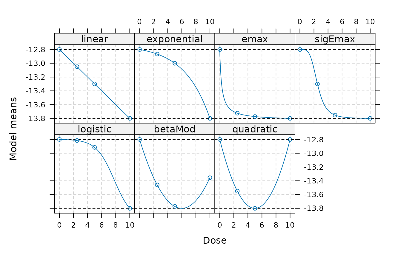
The mods object we just created above contains the full
model parameters, which can be helpful for understanding how the
guesstimates are translated onto the parameter scale.
display_params_table(mods)| Name | Value | |
|---|---|---|
| linear | linear | {e0=-12.8, delta=-0.1} |
| exponential | exponential | {e0=-12.8, e1=-0.0666665802154335, delta=3.60673602074522} |
| emax | emax | {e0=-12.8, eMax=-1.02777777777778, ed50=0.277777777777778} |
| sigEmax | sigEmax | {e0=-12.8, eMax=-1.00277008310249, ed50=2.5, h=4.24792751344358} |
| logistic | logistic | {e0=-12.7974358974359, eMax=-1.17948717948718, ed50=7.79415312704722, delta=1.27167389072021} |
| betaMod | betaMod | {e0=-12.8, eMax=-1, delta1=1, delta2=1} |
| quadratic | quadratic | {e0=-12.8, b1=-0.4, b2=0.04} |
And we can see the assumed treatment effects for the specified dose groups below:
| linear | exponential | emax | sigEmax | logistic | betaMod | quadratic | |
|---|---|---|---|---|---|---|---|
| 0 | -12.80 | -12.80000 | -12.80000 | -12.80000 | -12.80000 | -12.80000 | -12.80 |
| 2.5 | -13.05 | -12.86667 | -13.72500 | -13.30138 | -12.81551 | -13.45972 | -13.55 |
| 5 | -13.30 | -13.00000 | -13.77368 | -13.75263 | -12.91538 | -13.77222 | -13.80 |
| 10 | -13.80 | -13.80000 | -13.80000 | -13.80000 | -13.80000 | -13.35556 | -12.80 |
Posterior Calculation
In the first step of Bayesian MCPMod, the posterior is calculated by combining the prior information with the estimated results of the trial (Fleischer F 2022).
posterior <- getPosterior(
  prior_list = prior_list,
  mu_hat     = trial_data$rslt,
  S_hat      = diag(trial_data$se^2),
  calc_ess   = TRUE
)

knitr::kable(summary(posterior))| mean | sd | 2.5% | 50.0% | 97.5% | |
|---|---|---|---|---|---|
| Ctr | -11.23854 | 0.6957444 | -12.56205 | -11.25389 | -9.831438 |
| DG_1 | -14.88114 | 0.7130817 | -16.27875 | -14.88114 | -13.483523 |
| DG_2 | -15.08015 | 0.7101057 | -16.47193 | -15.08015 | -13.688367 |
| DG_3 | -15.63659 | 0.7259755 | -17.05948 | -15.63659 | -14.213707 |
Bayesian MCPMod Test Step
The testing step of Bayesian MCPMod is executed using a critical value on the probability scale and a pseudo-optimal contrast matrix.
The critical value is calculated using (re-estimated) contrasts for frequentist MCPMod to ensure error control when using weakly-informative priors.
A pseudo-optimal contrast matrix is generated based on the variability of the posterior distribution (see (Fleischer F 2022) for more details).
set.seed(7015) # re-sets seed only for this example; remove in your analysis script
crit_pval <- getCritProb(
  mods           = mods,
  dose_levels    = dose_levels,
  cov_new_trial  = diag(trial_data$se^2),
  alpha_crit_val = 0.05
)

contr_mat <- getContr(
  mods          = mods,
  dose_levels   = dose_levels,
  cov_posterior = diag(summary(posterior)[, 2]^2)
)
Please note that there are different ways to derive the contrasts. The following code shows the implementation of some of these ways but it is not executed and the contrast specification above is used.
# i) the frequentist contrast
contr_mat_prior <- getContr(
  mods           = mods,
  dose_levels    = dose_levels,
  dose_weights   = n_patients,
  prior_list     = prior_list)
# ii) re-estimated frequentist contrasts
contr_mat_prior <- getContr(
  mods           = mods,
  dose_levels    = dose_levels,
  cov_new_trial  = diag(trial_data$se^2))
# iii)  Bayesian approach using number of patients for new trial and prior distribution
contr_mat_prior <- getContr(
  mods           = mods,
  dose_levels    = dose_levels,
  dose_weights   = n_patients,
  prior_list     = prior_list)
The Bayesian MCP testing step is then executed:
BMCP_result <- performBayesianMCP(
  posterior_list = posterior,
  contr          = contr_mat,
  crit_prob_adj  = crit_pval)
Summary information:
BMCP_result## Bayesian Multiple Comparison Procedure
## Significant: 1
## Critical Probability: 0.9845439
## Maximum Posterior Probability: 0.9999999
## Posterior Probabilities for Model Shapes
## lin exp emax sigE log betaM quad
## Posterior Prob 0.9999651 0.9983173 0.9999999 0.9999988 0.9956910 0.9999942 0.9894574
## Significant 1 1 1 1 1 1 1
## Average Posterior ESS
## Dose Level: Ctr DG_1 DG_2 DG_3
## Avg Post ESS: 197.2 186.6 188.2 180.0The testing step is significant, indicating a non-flat dose-response
shape. All models are significant, with the emax model
indicating the greatest deviation from the null hypothesis.
Model Fitting and Visualization
In the model fitting step the posterior distribution is used as basis.
Both simplified and full fitting are performed.
For the simplified fit, the multivariate normal distribution of the control group is approximated and reduced by a one-dimensional normal distribution.
The actual fit (on this approximated posterior distribution) is then
performed using generalized least squares criterion. In contrast, for
the full fit, the non-linear optimization problem is addressed via the
Nelder-Mead algorithm (Wikipedia 2024)
implemented by the nloptr package.
The output of the fit includes information about the predicted effects for the included dose levels, the generalized AIC, and the corresponding weights.
For the considered case, the simplified and the full fit are very similar, so we present the full fit.
# If simple = TRUE, uses approx posterior
# Here we use complete posterior distribution
model_fits <- getModelFits(
  models      = mods,
  dose_levels = dose_levels,
  posterior   = posterior,
  simple      = FALSE)
Estimates for dose levels not included in the trial:
| Name | Value | |
|---|---|---|
| avgFit | avgFit | -11.320, -14.682, -15.132, -15.313, -15.518, -15.532 |
| betaMod | betaMod | -11.270, -14.787, -15.098, -15.246, -15.450, -15.556 |
| emax | emax | -11.268, -14.805, -15.133, -15.257, -15.408, -15.529 |
| exponential | exponential | -12.637, -13.395, -13.898, -14.254, -15.023, -16.330 |
| linear | linear | -12.453, -13.431, -14.017, -14.408, -15.191, -16.364 |
| logistic | logistic | -11.269, -14.836, -15.273, -15.352, -15.390, -15.396 |
| quadratic | quadratic | -11.506, -14.112, -15.164, -15.652, -16.117, -15.537 |
| sigEmax | sigEmax | -11.268, -14.810, -15.092, -15.217, -15.394, -15.566 |
Plots of fitted dose-response models and an AIC-based average model:
plot(model_fits)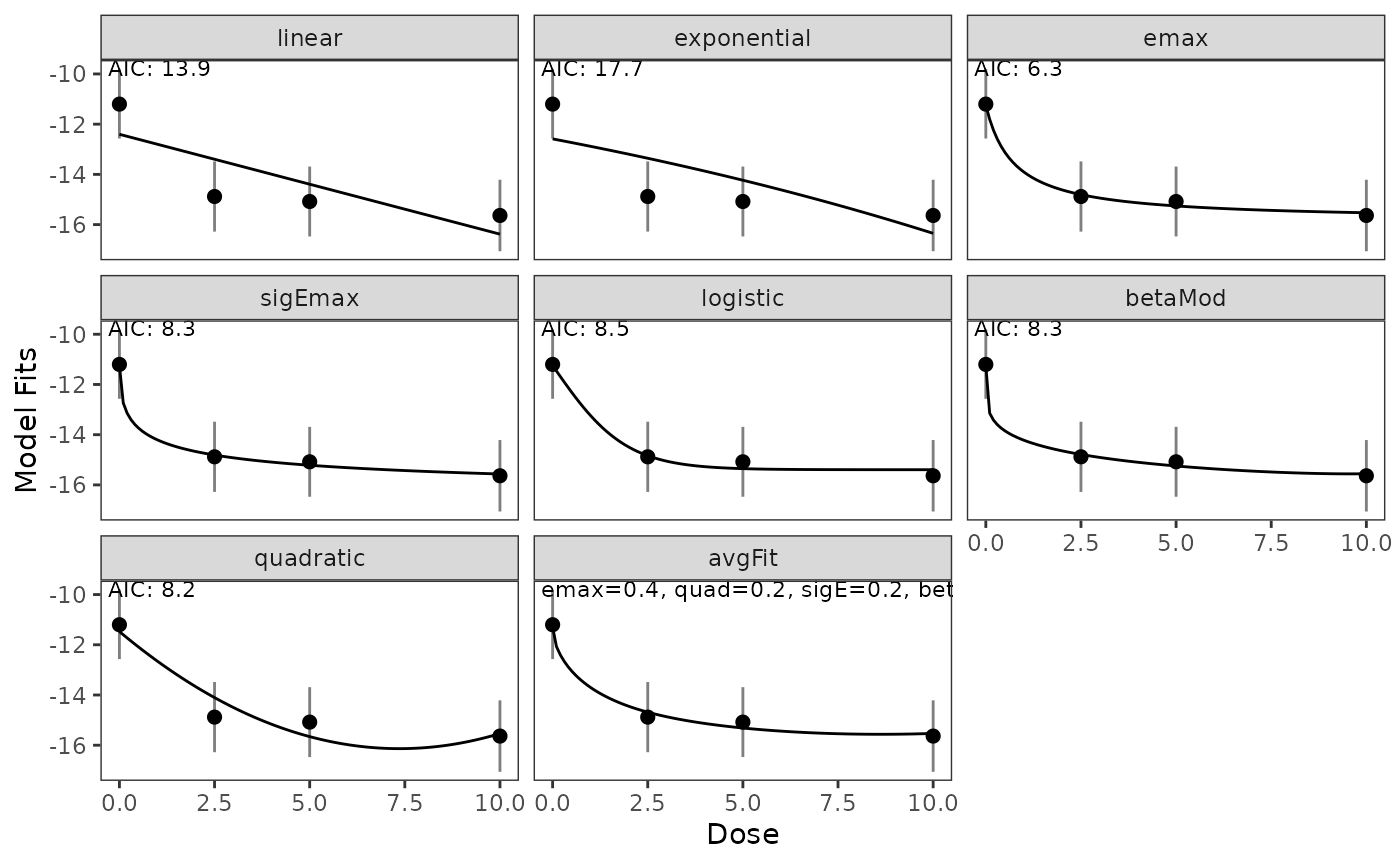
To assess the uncertainty, one can additionally visualize credible bands (orange shaded areas, default levels are 50% and 95%).
These credible bands are calculated with a bootstrap method as follows:
Samples from the posterior distribution are drawn and for every sample the simplified fitting step and a prediction is performed.
These predictions are then used to identify and visualize the specified quantiles.
plot(model_fits, cr_bands = TRUE)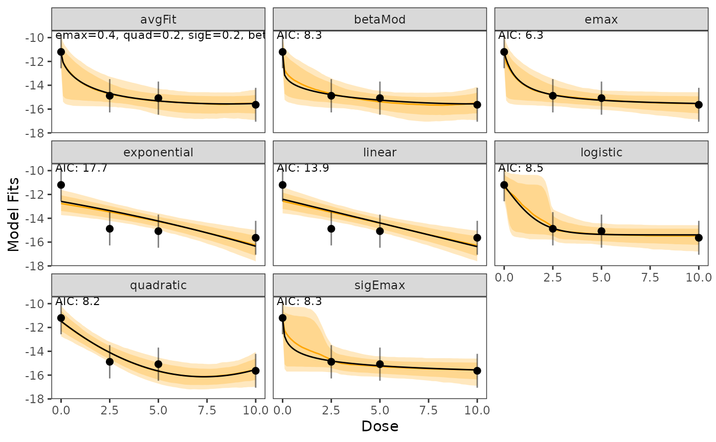
The bootstrap-based quantiles can also be directly calculated via the
getBootstrapQuantiles() function and a sample from the
model fits can bootstrapped using
getBootstrapSamples().
For this example, only 10 samples are bootstrapped for each model fit.
set.seed(7015) # re-sets seed only for this example; remove in your analysis script
bootstrap_quantiles <- getBootstrapQuantiles(
  model_fits = model_fits,
  quantiles  = c(0.025, 0.5, 0.975),
  doses      = c(0, 2.5, 4, 5, 7, 10),
  n_samples  = 10)
The bootstrap quantiles include information about the absolute quantiles (sample_type=abs) and also about the placebo-adjusted (resp. control-adjusted) quantiles (sample_type=diff).
reactable::reactable(
  data = bootstrap_quantiles |>
    tidyr::pivot_wider(names_from = q_prob, values_from = q_val),
  groupBy = "model",
  columns = list(
    dose    = colDef(format = list(aggregated = colFormat(suffix = " dose"))),
    "0.025" = colDef(format = list(cell = colFormat(digits = 4))),
    "0.5"   = colDef(format = list(cell = colFormat(digits = 4))),
    "0.975" = colDef(format = list(cell = colFormat(digits = 4)))
  )
)
Technical note: The median quantile of the bootstrap based procedure is not necessary similar to the main model fit, as they are derived via different procedures.
The main fit (black line) minimizes residuals for the posterior distribution, while the bootstrap median is the median fit of random sampling.
Assessment of the Minimally Efficacious Dose
The Minimally Efficacious Dose (MED) per model shape can be assessed
with the function getMED().
getMED(
  delta       = 4,
  model_fits  = model_fits,
  dose_levels = seq(min(dose_levels), max(dose_levels), by = 0.01))
## avgFit betaMod emax exponential linear logistic quadratic sigEmax
## med_reached 1.00 1.0 1.00 0 0 1.00 1.00 1.0
## med 5.05 5.2 5.12 NA NA 3.97 4.67 5.5For an optional Bayesian decision rule for the MED assessment and
further details, please see ?getMED().
Additional Note
Testing, modeling, and MED assessment can also be combined via
performBayesianMCPMod():
performBayesianMCPMod(
  posterior_list   = posterior,
  contr            = contr_mat,
  crit_prob_adj    = crit_pval,
  delta            = 4,
  simple           = FALSE)