A User Guide for the `endpoints` Package

Colin Longhurst

2026-04-14

library(endpoints)
library(tidyverse)

Introduction

The makeData() framework is designed to simulate flexible clinical trial datasets with a mix of endpoint types and trial-design features, while keeping the interface simple and modular. It supports both straightforward single-endpoint simulations and more complex multivariate settings with correlated outcomes generated through a Gaussian copula (NORTA-style) construction. The function also accommodates:

• trials with multiple treatment arms
• time-to-event outcomes with censoring (competing or semi-competing risks)
• realistic trial logistics such as stochastic enrollment and administrative follow-up

In this vignette, we illustrate the package through a sequence of examples, beginning with simple single-endpoint simulations and gradually introducing more advanced features.

Quick Start: One Endpoint Simulations

The core function in endpoints is makeData(), which is used across all simulation settings. In the simplest case, makeData() can simulate a single-endpoint trial with one or more treatment arms.

For one-endpoint simulations, the most important arguments are:

• sample_size_per_group: Sample size per treatment arm (scalar or vector)
• endpoint_details: A list of endpoint specifications (one sub-list per endpoint)

An optional argument used in multivariate settings is:

• correlation_matrix: A correlation matrix describing dependence across endpoints

This is discussed in later sections.

makeData(correlation_matrix = NULL,
  sample_size_per_group = 1000,
  endpoint_details = list(
    ...
    )
  )

Specifying endpoints endpoint_details

The makeData() function allows for four endpoint types, which are encoded via the endpoint_details argument: continuous, binary, count and time-to-event. We discuss each below.

Continuous

An example specification of a continuous endpoint is seen below:

c_ep1 <- list(
      endpoint_type = "continuous",
      baseline_mean = 10,
      sd            = c(3,2),
      trt_effect    = -2
    )

When generating continuous endpoints, makeData() uses a Gaussian (normal) marginal distribution. The endpoint specification arguments are:

• baseline_mean: Mean in the control group.
• sd: If a scalar is provided, a common SD is used across groups. If a vector is provided, it specifies arm-specific SDs.
• trt_effect = NULL: Mean difference(s) for treatment group(s) relative to control. A scalar is used for one treatment arm; a vector may be used for multiple treatment arms. If NULL, only control-group data are generated.

For a two-arm study, trt_effect = -2 implies treatment mean = baseline_mean - 2

simple1 <- makeData(correlation_matrix = NULL,
  sample_size_per_group = 1000,
  SEED = 1,
  endpoint_details = list(c_ep1)
  )

A quick summary of the simulation details is displayed when printing the resulting object:

simple1

## <makeDataSim>
##   n =2000
##   n_arms =2
##   endpoints =1
##   target_correlation =FALSE
##   single_endpoint_mode =TRUE
##   control_only =FALSE
##   n_by_arm = 0:1000, 1:1000
##   endpoint_types = continuous
## 
##   data (head):
##             Cont_1 trt
## 1 8.12063857862128   0
## 2  9.0212999043454   0
## 3 10.5509299725547   0
## 4 13.9893977783661   0
## 5 7.49311413608736   0
## ⋮                ⋮   ⋮

To confirm the distributions have the correct parameters, we can use the summary function

knitr::kable(summary(simple1)$continuous)

endpoint	arm	input_baseline_mean	input_sd	input_trt_effect	est_baseline_mean	est_trt_effect	est_resid_sd
Cont_1	0	10	3	0	10.02815	0.000000	2.999293
Cont_1	1	10	2	-2	10.02815	-2.102053	2.066130

From above, we see that the estimated baseline mean, treatment effect and standard deviation parameter are all close to the true values.

The resulting simulated data set can be accessed from the main makeDataSim object:

head(simple1$data)

##      Cont_1 trt
## 1  8.120639   0
## 2  9.021300   0
## 3 10.550930   0
## 4 13.989398   0
## 5  7.493114   0
## 6 13.817288   0

The response variable is automatically encoded as Cont_1 to indicate that it is the first continuous endpoint.

Binary

For binary outcomes, the event probability is modeled on the logit scale. You may specify treatment effects either directly on the probability scale (trt_prob) or on the log-odds scale (trt_effect), but not both.

bin_ep1 <- list(
      endpoint_type  = "binary",
      baseline_prob  = 0.30,
      trt_prob = 0.45
    )

Binary endpoints are specified via the following arguments:

• baseline_prob: Probability of success in the control group.
• trt_prob: Scalar or vector of treatment-group success probabilities.
• trt_effect = NULL: Optional scalar or vector of treatment effects on the log-odds scale (relative to control). Only one of trt_prob or trt_effect may be supplied.

Once again we can confirm that the simulated data has the proper characteristics:

simple2 <- makeData(correlation_matrix = NULL,
  sample_size_per_group = 1000,
  SEED = 2,
  endpoint_details = list(bin_ep1)
  )
knitr::kable(summary(simple2)$binary)

endpoint	arm	input_baseline_prob	input_trt_logOR	input_trt_prob	est_baseline_prob	est_trt_logOR	est_prob
Bin_1	0	0.3	0.0000000	0.30	0.302	0.000000	0.302
Bin_1	1	0.3	0.6466272	0.45	0.302	0.641161	0.451

Count

To generate count outcomes, we use the zero-inflated negative binomial distribution with a log-link function. The parameterization arguments are as follows:

int_ep1 <- list(
      endpoint_type = "count",
      baseline_mean = 8,    
      trt_count = 10,
      size          = 100, # approximate Poisson       
      p_zero        = 0     
    )

• baseline_mean: Mean count in the control group.
• trt_count: Scalar or vector of treatment-group mean counts.
• trt_effect = NULL: Optional scalar or vector of treatment effects on the log rate-ratio scale. Only one of trt_count or trt_effect may be supplied.
• size: Negative binomial dispersion parameter (larger values reduce overdispersion and approach the Poisson limit). In the parameterization used, the variance of the distribution is equal to \(\mu + \frac{\mu^2}{\phi}\). Here, size controls \(\phi\).
• p_zero: Zero-inflation probability.

An example use can be seen below:

simple3 <- makeData(correlation_matrix = NULL,
  sample_size_per_group = 1000,
  SEED = 2,
  endpoint_details = list(int_ep1)
  )
knitr::kable(summary(simple3)$count)

endpoint	arm	input_baseline_mean	input_trt_logRR	input_trt_mean	input_size	input_p_zero	est_baseline_mean	est_trt_logRR	est_size	obs_mean	obs_p0
Int_1	0	8	0.0000000	8	100	0	7.987	0.0000000	54.55504	7.987	0
Int_1	1	8	0.2231436	10	100	0	7.987	0.2321426	54.55504	10.074	0

Note: When size is large, the negative binomial approaches a Poisson distribution. In those cases, the dispersion parameter may be difficult to estimate precisely from a single simulated dataset (e.g., via MASS::glm.nb()), which is usually not a practical concern for simulation.

Time-to-Event Endpoints

Time-to-event endpoints are supported through exponential event-time models with optional independent censoring, fatal/non-fatal event logic, administrative censoring, and stochastic enrollment. We defer details to the dedicated section below.

Multiple Treatment Arms

To extend the above simulations to settings with several treatment groups, we can simply replace scalar inputs with vectors. In general, if there are \(G\) total study arms (including control), then treatment-specific vectors (e.g., trt_prob, trt_effect, sd) should typically have length \(G-1\), corresponding to the non-control arms in order.

For example, imagine we have a 4-grp study with a binary endpoint:

bin_4grp <- list(
      endpoint_type  = "binary",
      baseline_prob  = 0.30,
      trt_prob = c(0.35, 0.40, 0.45)
    )

sim_bin4grp <- makeData(correlation_matrix = NULL,
  sample_size_per_group = c(100,200,400,400),
  SEED = 123,
  endpoint_details = list(bin_4grp)
  )
sim_bin4grp

## <makeDataSim>
##   n =1100
##   n_arms =4
##   endpoints =1
##   target_correlation =FALSE
##   single_endpoint_mode =TRUE
##   control_only =FALSE
##   n_by_arm = 0:100, 1:200, 2:400, 3:400
##   endpoint_types = binary
## 
##   data (head):
##   Bin_1 trt
## 1     0   0
## 2     1   0
## 3     0   0
## 4     1   0
## 5     1   0
## ⋮     ⋮   ⋮

Once again we can ensure the distributions are being simulated correctly by calling summary:

knitr::kable(summary(sim_bin4grp)$binary)

endpoint	arm	input_baseline_prob	input_trt_logOR	input_trt_prob	est_baseline_prob	est_trt_logOR	est_prob
Bin_1	0	0.3	0.0000000	0.30	0.29	0.0000000	0.290
Bin_1	1	0.3	0.2282587	0.35	0.29	0.1871990	0.330
Bin_1	2	0.3	0.4418328	0.40	0.29	0.4690414	0.395
Bin_1	3	0.3	0.6466272	0.45	0.29	0.6744902	0.445

Correlated Endpoints with Gaussian Copula

Gaussian copulas provide a flexible way to generate multivariate outcomes with user-specified marginal distributions and dependence. Let \(\mathbf{Z} = (Z_1,\dots,Z_J)^\top \sim \mathrm{MVN}(\mathbf{0}, \Sigma_Z)\). Applying the probability integral transform componentwise gives

\[ X_j = F_j^{-1}\{\Phi(Z_j)\}, \qquad j=1,\dots,J, \]

where \(\Phi\) is the standard normal CDF and \(F_j^{-1}\) is the inverse CDF (quantile function) of the desired marginal distribution for endpoint \(j\). This construction preserves the chosen marginals and induces dependence across endpoints through the Gaussian copula.

Because Pearson correlation is generally not preserved under nonlinear monotone transformations, makeData() optionally uses numerical calibration (target_correlation = TRUE) to find a latent Gaussian correlation matrix that approximately reproduces the requested Pearson correlation matrix on the observed endpoint scale.

Important: When target_correlation = FALSE, the supplied correlation_matrix is used directly as the latent Gaussian correlation matrix (the copula parameter), not as a calibrated Pearson correlation matrix on the observed endpoint scale. It is recommended that this option is set to TRUE. See Cario & Nelson (1997) for more details.

Creating the Correlation Matrix

To create a correlation matrix, we use the corr_make() function which has two arguments:

• num_endpoints: The number of correlated endpoints to generate
• values: Pairwise correlations specified as a 3-column object (e.g., matrix or data frame), where each row has the form (i, j, rho) giving the correlation between endpoints i and j. Unspecified pairs default to a correlation value of 0.

Consider a trial with 3 endpoints with the following correlation:

corMat_3 <- corr_make(
  num_endpoints =   3,
  values = rbind(
    c(1,2,.2), c(1,3,.1),
    c(2,3,.15)
  )
) 

Simulating Correlated Endpoints

Using the endpoints defined above, we can now generate a trial with three correlated endpoints, one continuous, one binary and one count:

sim_3eps <- makeData(
  correlation_matrix    = corMat_3,
  sample_size_per_group = 3000,
  SEED = 777,
  endpoint_details = list(
    c_ep1,
    bin_ep1,
    int_ep1
  )
)

To quickly confirm that the estimated correlation between endpoints is close to the correlation specified, we use the summary function:

Show summary(sim_3eps)

n_arms: 2 

Target correlation:
     [,1] [,2] [,3]
[1,]  1.0 0.20 0.10
[2,]  0.2 1.00 0.15
[3,]  0.1 0.15 1.00

Estimated correlation (by arm):

arm_0:
       Cont_1 Bin_1 Int_1
Cont_1  1.000 0.194 0.122
Bin_1   0.194 1.000 0.129
Int_1   0.122 0.129 1.000

arm_1:
       Cont_1 Bin_1 Int_1
Cont_1  1.000 0.222 0.076
Bin_1   0.222 1.000 0.154
Int_1   0.076 0.154 1.000

Continuous endpoints (endpoint x arm):
  endpoint arm input_baseline_mean input_sd input_trt_effect est_baseline_mean
1   Cont_1   0                  10        3                0          10.05584
2   Cont_1   1                  10        2               -2          10.05584
  est_trt_effect est_resid_sd
1       0.000000     2.986202
2      -2.058158     1.993636

Binary endpoints (endpoint x arm):
  endpoint arm input_baseline_prob input_trt_logOR input_trt_prob
1    Bin_1   0                 0.3       0.0000000           0.30
2    Bin_1   1                 0.3       0.6466272           0.45
  est_baseline_prob est_trt_logOR  est_prob
1             0.297     0.0000000 0.2970000
2             0.297     0.6945707 0.4583333

Count endpoints (endpoint x arm):
  endpoint arm input_baseline_mean input_trt_logRR input_trt_mean input_size
1    Int_1   0                   8       0.0000000              8        100
2    Int_1   1                   8       0.2231436             10        100
  input_p_zero est_baseline_mean est_trt_logRR est_size  obs_mean       obs_p0
1            0          8.070667     0.0000000 150.3706  8.070667 0.0006666667
2            0          8.070667     0.2223502 150.3706 10.080333 0.0000000000

From the summary above, we see that the within-arm correlation is close to that specified in corMat_3 and that the marginal distributions have the correct distributional characteristics. Note that because the correlation calibration is numerical (and summaries are based on finite samples), small discrepancies between the requested and empirical within-arm correlations are expected.

Here we also introduce the plot function, which allows users to quickly confirm simulation details:

plot(sim_3eps)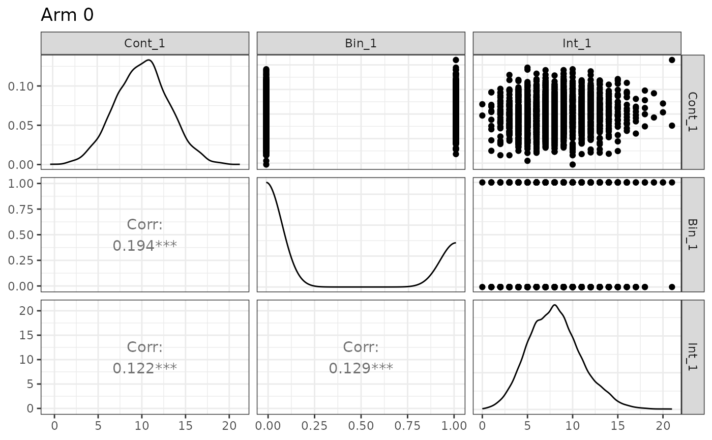

Note that different experimental arms can be plotted by toggling the arm argument, and that names may also be supplied:

plot(sim_3eps,arm=1,names=c("BMI","Illness Worsened","# episodes"))

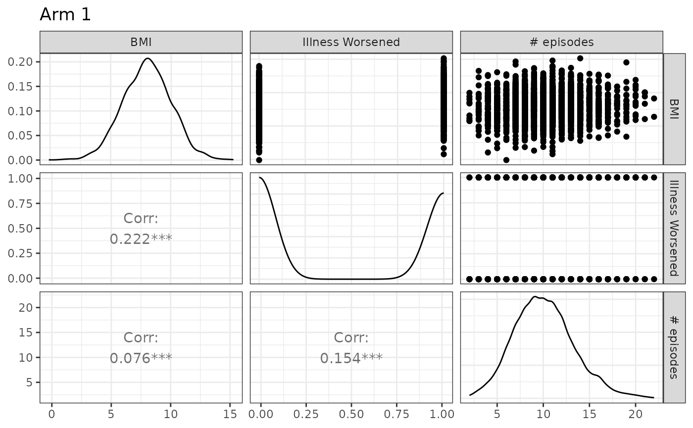
The code can easily be modified to accommodate several treatment groups by applying the conventions discussed in the previous section.

Time-to-event Endpoints and Censoring

In makeData(), all time-to-event (TTE) endpoints are distributed as exponential random variables \(f(x;\lambda) = \lambda e^{-\lambda x}\). They are encoded as elements in endpoint_details as follows:

• baseline_rate: The exponential event-rate parameter \(\lambda\) for the control group (so the mean event time is \(1/\lambda\)).
• trt_effect: Scalar or vector of treatment effects on the log hazard-ratio scale.
• censoring_rate = NULL: Exponential censoring-rate parameter for independent censoring (if NULL, no random censoring is applied).
• fatal_event: If TRUE, the endpoint is treated as fatal and censors subsequent non-fatal TTE endpoints. See below for details.

tte_ep1 <- list(
      endpoint_type  = "tte",
      baseline_rate  = 1/24,        
      trt_effect     = log(0.80),   
      censoring_rate = NULL,        
      fatal_event    = F     
    )

Censoring

For a time-to-event endpoint, for the \(i^{th}\) patient we observe \(X_i = \min\{T_i, C_i\}\) where \(T \sim Exp(\lambda_e)\) is the event time and \(C_i \sim Exp(\lambda_c)\) is the censoring time. For the primary terminal event (or a non-terminal event when there are no terminal events), the probability of observing an event is \[P({T}_i < {C}_i) = \int^\infty_0\lambda_ee^{-\lambda_ex}e^{-\lambda_cx} = \frac{\lambda_{e}}{\lambda_e+\lambda_c},\]

which can be used to select a censoring rate that produces the user-specified event rate. In the example from the code chunk above, if we want to select a censoring rate such that we observe an event rate of .9, some algebra yields \(\lambda_c = \frac{1/24}{0.90} -\frac{1}{24} = 1/216\). This can be calculated by using the helper function rate_from_prob():

lambda_c <- rate_from_prob(
  target_prob = 0.90, # target proportion of patients with events
  mode = "simple", 
  event_rate = 1 / 24 # rate parameter for primary event
)
print(paste0("1","/",1/lambda_c))

## [1] "1/216"

When there are semi-competing risks, and the TTE endpoints have low correlation, the event rate for the secondary, non-fatal TTE endpoint can be approximated as \(\frac{\lambda_{e2}}{\lambda_{e1}+\lambda_{c1}+\lambda_{e2}+\lambda_{c2}}\) where the subscripts \(1, 2\) denote the first and secondary endpoints. The above formula is meant only as an approximation as the dependence (induced by the copula) between \(X_1\) and \(X_2\) is not accounted for. This approximation can also be handled by the helper function. In this case, the output is the rate of the censoring mechanism for the secondary endpoint.

rate_from_prob(
  target_prob = 0.20, # hypothetical example
  mode = "semi-competing",
  fatal_event_rate = 1 / 50,
  fatal_censor_rate = 1 / 16.667,
  nonfatal_event_rate = 1 / 35
)

## [1] 0.03428691

Please see ?rate_from_prob() for details.

We also note here that the censoring mechanism is independent of the copula so pairwise correlations involving censored TTE endpoints generally will not equal the specified coefficient. To confirm the simulation is working as intended, we recommend first simulating the data without censoring, confirming the correlation, then re-generating the data with censoring.

Fatal Events

Let \(X_1\) be a fatal event and \(X_2\) be a non-fatal event, then we write \(X_2 = \min\{T_1, C_1, T_2,C_2\}\). That is, we cannot observe any event that occurs after a fatal event occurs or is censored.

If a non-fatal event occurs before a fatal event (\(T_2 < \{T_1, C_1,C_2\}\)), a fatal event can still be subsequently observed (or censored). If a non-fatal event is censored before a fatal event (\(C_2 < \{T_1, C_1,T_2\}\)), a fatal event can still be subsequently observed (or censored), unless non_fatal_censors_fatal = TRUE is toggled in the main makeData() function. This is a global option for all TTEs simulated.

Semi-Competing Risks Example

We want to generate a data set with TTE endpoints, one fatal and one non-fatal. The fatal event has an average time of 50 in the control group, and 60 in the treatment group. We want an observed event rate of .25 in the control group.

To solve for the needed log hazard ratio, we solve \(\frac{1}{60} = \frac{1}{50} \cdot HR \to \text{HR} = .833\). To solve for the censoring rate, we solve \(\frac{1/50}{0.25} - \frac{1}{50} = 1/ 16.667\).

For the second endpoint, we want a mean time of 35 for control group and 45 for treatment group, with an observed event rate of .45 for the control group. To solve for the needed log hazard ratio, we solve \(\frac{1}{45} = \frac{1}{35} \cdot HR \to \text{HR} = 0.778\). To solve for the censoring rate, we solve \(\frac{1/35}{0.45} - \frac{1}{35} = 1/ 28.64\).

We assume a correlation of .2 between the endpoints.

tte_fatal <-  list(
      endpoint_type  = "tte",
      baseline_rate  = 1/50,        
      trt_effect     = log(0.8333),   
      censoring_rate = 1/16.667,        
      fatal_event    = TRUE   
    ) 

tte_nonfatal <- list(
      endpoint_type  = "tte",
      baseline_rate  = 1/35,        
      trt_effect     = log(0.778),   
      censoring_rate = 1/28.64,        
      fatal_event    = FALSE 
    ) 

small_cor <- corr_make(
  num_endpoints = 2,
  values = rbind( c(1,2, 0.20)) # correlation
)

tte_ex <- makeData(
  correlation_matrix    = small_cor,
  sample_size_per_group = 5000,
  SEED = 321,
  endpoint_details = list( tte_fatal, tte_nonfatal),
  non_fatal_censors_fatal = FALSE
)
tte_ex

## <makeDataSim>
##   n =10000
##   n_arms =2
##   endpoints =2
##   target_correlation =TRUE
##   single_endpoint_mode =FALSE
##   control_only =FALSE
##   n_by_arm = 0:5000, 1:5000
##   endpoint_types = time-to-event, time-to-event
## 
##   data (head):
##               TTE_1             TTE_2 trt Status_1 Status_2
## 1  1.04727950385236  1.04727950385236   0        0        0
## 2  1.08654899491183  1.08654899491183   0        0        0
## 3  28.7011752270296  10.1710911152606   0        0        1
## 4   7.0854601196209  1.40421959333994   0        0        1
## 5 0.743645541628904 0.743645541628904   0        0        0
## ⋮                 ⋮                 ⋮   ⋮        ⋮        ⋮

And we can confirm our inputs:

Show summary(tte_ex)

n_arms: 2 

Target correlation:
     [,1] [,2]
[1,]  1.0  0.2
[2,]  0.2  1.0

Estimated correlation (by arm):

arm_0:
      TTE_1 TTE_2
TTE_1 1.000 0.568
TTE_2 0.568 1.000

arm_1:
      TTE_1 TTE_2
TTE_1 1.000 0.621
TTE_2 0.621 1.000

TTE endpoints (endpoint x arm):
  endpoint arm censor_col input_baseline_rate input_trt_logHR input_trt_HR
1    TTE_1   0   Status_1          0.02000000       0.0000000       1.0000
2    TTE_1   1   Status_1          0.02000000      -0.1823616       0.8333
3    TTE_2   0   Status_2          0.02857143       0.0000000       1.0000
4    TTE_2   1   Status_2          0.02857143      -0.2510288       0.7780
  est_trt_logHR est_trt_HR obs_event_rate   exp_rate
1     0.0000000  1.0000000         0.2498 0.01993274
2    -0.1826152  0.8330887         0.2168 0.01665117
3     0.0000000  1.0000000         0.1852 0.02619647
4    -0.2191347  0.8032135         0.1616 0.02094082

We emphasize once again that censoring and the presence of competing risks can alter correlation (estimated vs expected) and marginal distribution parameters. As mentioned before, we recommend first generating data with no censoring or fatal events to confirm the overall structure before introducing those elements.

In the summary() output for simulated TTE endpoints, the column exp_rate reports the arm-specific exponential maximum likelihood estimate (MLE) of the event rate, computed from the observed times and event indicators after censoring/fatal-event logic has been applied. For a given arm, this is

\[ \widehat{\lambda}_{\text{exp}} = \frac{\sum_i \delta_i}{\sum_i X_i}, \]

where \(X_i\) is the observed follow-up time for subject \(i\) (possibly censored), and \(\delta_i\in\{0,1\}\) is the event indicator (1 = event observed, 0 = censored).

This is the standard MLE for an exponential survival model with right censoring. In the summary output:

• obs_event_rate is the observed proportion of subjects with an event (i.e., \(\bar\delta\)),
• exp_rate is the exponential rate estimate \(\sum \delta_i / \sum X_i\),
• est_trt_logHR is the treatment log-hazard ratio estimated from a Cox model fit.

These quantities are related but not identical. In particular, exp_rate is a descriptive arm-level estimator under an exponential model assumption, while est_trt_logHR comes from a semi-parametric Cox model.

Because censoring, administrative censoring, and fatal-event truncation modify the observed follow-up times and event indicators, the estimated exp_rate may differ from the user-specified baseline_rate (and implied treatment-group rates), especially in small samples or when censoring is heavy.

In this example, the arm-specific exp_rate values are close to the data-generating exponential event rates (approximately \(1 / 50,1 / 60,1 / 35\), and \(1 / 45\) ), which is expected here because the sample size is large and censoring is independent; even though censoring changes the observed event proportion, the exponential MLE \(\sum \delta_i / \sum X_i\) remains a consistent estimator of the event hazard under the exponential model.

Administrative Censoring & Stochastic Enrollment

Administrative Censoring

Administrative censoring (which we denote as \(\mathcal{A}\)) is controlled via enrollment_details argument, which is a list of settings. Within enrollment_details administrative censoring is toggled using administrative_censoring = NULL. If it is set to a positive value, then any TTE event that occurs (or is censored) after \(\mathcal{A}\), is set to \(\mathcal{A}\) as that is the limit of follow-up.

To illustrate, we can re-run the example above, but this time setting a 24 time-unit limit:

 tte_ex_admin_cens <- makeData(
  correlation_matrix    = small_cor,
  sample_size_per_group = 5000,
  SEED = 321,
  endpoint_details = list( tte_fatal, tte_nonfatal),
  enrollment_details = list(
    administrative_censoring = 24
  ),
  non_fatal_censors_fatal = FALSE
)

Comparing the datasets, we now see patient 3 is administratively censored at time 24:

head(tte_ex$data) %>% knitr::kable(.,caption = "Data without admin censoring")

Data without admin censoring

TTE_1	TTE_2	trt	Status_1	Status_2
1.0472795	1.0472795	0	0	0
1.0865490	1.0865490	0	0	0
28.7011752	10.1710911	0	0	1
7.0854601	1.4042196	0	0	1
0.7436455	0.7436455	0	0	0
18.4536996	7.1912254	0	1	0

head(tte_ex_admin_cens$data) %>% knitr::kable(.,caption = "Data with admin censoring")

Data with admin censoring

TTE_1	TTE_2	trt	Status_1	Status_2	enrollTime
1.0472795	1.0472795	0	0	0	0
1.0865490	1.0865490	0	0	0	0
24.0000000	10.1710911	0	0	1	0
7.0854601	1.4042196	0	0	1	0
0.7436455	0.7436455	0	0	0	0
18.4536996	7.1912254	0	1	0	0

Note that an enrollTime column is automatically generated when using this feature.

If there is no non-administrative censoring (e.g. no random drop-out), we can solve for expected event rates by evaluating \(\int_{0}^{\mathcal{A}} \lambda e^{-\lambda x} dx = 1 - e^{-\lambda x}\). To solve for \(\lambda\), we calculate \(\frac{\ln(1-r)}{-\mathcal{A}}\) where r is the desired event rate. For example, if we want to simulate a 4-year trial with a 20% fatal event rate, we need to set the baseline hazard to log(1-.2)/(-4) = .0558. Once again, we can use the helper function rate_from_prob() to solve this math:

rate_from_prob(
  target_prob = 0.20,
  mode = "admin",
  admin_time = 4
)

## [1] 0.05578589

which can then be used in makeData()

admin_ex2 <- makeData(
  correlation_matrix    = NULL,
  sample_size_per_group = 5000,
  SEED = 12,
  endpoint_details = list( 
    list(
      endpoint_type  = "tte",
      baseline_rate  = .0558,        
      trt_effect     = 0,   
      fatal_event    = TRUE ) ),
  enrollment_details = list(
    administrative_censoring = 4
  ),
  non_fatal_censors_fatal = FALSE
)
obs_rates <- summary(admin_ex2)$tte$obs_event_rate
print(paste0("Observed event rate for control group is: ", round(obs_rates[1],2)))

## [1] "Observed event rate for control group is: 0.2"

Stochastic Enrollment

By default, all patients are enrolled on day 0 of the trial. To simulate a more realistic trial, probabilistic enrollment is controlled via the following arguments:

• enrollment_distribution = c("none","uniform","exponential","piecewise"): This specifies the enrollment-time distribution (default is "none"). If "uniform", enrollment time is \(\mathbf{U}[0,\mathcal{A}]\), where \(\mathcal{A}\) is the time of administrative censoring. If "exponential", enrollment time is based on an exponential distribution (see enrollment_exponential_rate). If "piecewise", enrollment follows a piecewise exponential distribution. This option requires specifying piecewise_enrollment_cutpoints and piecewise_enrollment_rates (see examples below).
• enrollment_exponential_rate = NULL: The rate for the exponential distribution if enrollment_distribution = "exponential".
• piecewise_enrollment_cutpoints = NULL: The time points defining the bins for the piecewise enrollment pattern.
• piecewise_enrollment_rates = NULL: The rates for each exponential distribution within each time bin.

If a user specifies stochastic enrollment and administrative censoring, then maximum potential time-on-study is \(\mathcal{A} - T_E\), where \(T_E\) is time of enrollment. If we re-run the example from above,

 tte_admin_cens_exp_enroll <- makeData(
  correlation_matrix    = small_cor,
  sample_size_per_group = 5000,
  SEED = 321,
  endpoint_details = list( tte_fatal, tte_nonfatal),
  enrollment_details = list(
    administrative_censoring = 24,
     enrollment_distribution = "exponential",
    enrollment_exponential_rate = 1/4
  ),
  non_fatal_censors_fatal = FALSE
)
knitr::kable(head(tte_admin_cens_exp_enroll$data),caption = "Data with admin censoring and stochastic enrollment")

Data with admin censoring and stochastic enrollment

TTE_1	TTE_2	trt	Status_1	Status_2	enrollTime
1.0472795	1.0472795	0	0	0	1.5548657
1.0865490	1.0865490	0	0	0	4.4949425
19.7241782	10.1710911	0	0	1	4.2758218
7.0854601	1.4042196	0	0	1	3.9579370
0.7436455	0.7436455	0	0	0	1.1697326
18.4536996	7.1912254	0	1	0	0.8527512

we now see that patient 3 is now censored at time 19.72 (instead of time 24), as their enrollment time is 4.28. From the code above, we observed an enrollment curve of:

ggplot2::ggplot(tte_admin_cens_exp_enroll$data, aes(x = enrollTime)) +
  geom_histogram(bins = 30,fill = "steelblue", alpha = 0.35,
    color = "black",linewidth = 0.3) +
  labs(
    x = "Enrollment time",
    y = "Count",
    title = "Histogram of enrollment times (Exponential)") +
  theme_bw()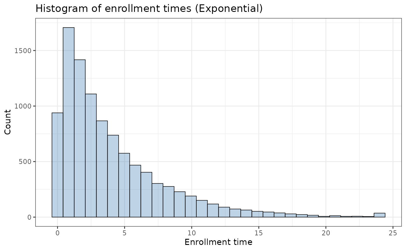

The function also supports a simple enrollment (uniform) curve:

ex_unif <- makeData(
  correlation_matrix    = small_cor,
  sample_size_per_group = 5000,
  SEED = 321321,
  endpoint_details = list( tte_fatal, tte_nonfatal),
  enrollment_details = list(
    administrative_censoring = 24,
     enrollment_distribution = "uniform"
  ),
  non_fatal_censors_fatal = FALSE
)

ggplot2::ggplot(ex_unif$data, aes(x = enrollTime)) +
  geom_histogram(bins = 30,fill = "steelblue", alpha = 0.35,
    color = "black",linewidth = 0.3) +
  labs(
    x = "Enrollment time",
    y = "Count",
    title = "Histogram of enrollment times (Uniform)") +
  theme_bw()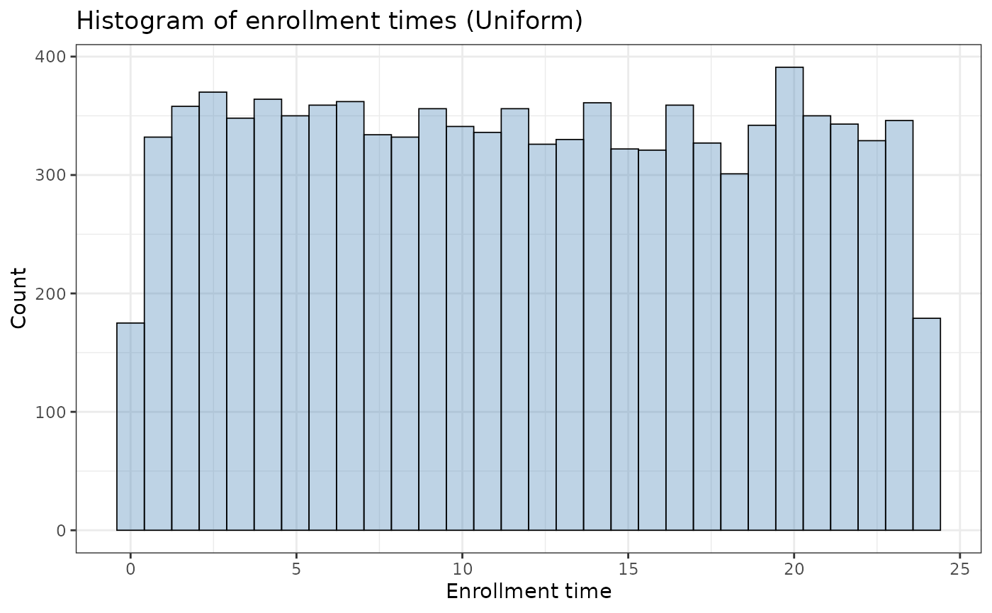

Stochastic enrollment does not change the underlying event-time generation mechanism (i.e., the event hazard parameters), but it can materially change observed follow-up time and observed event proportions when administrative censoring is present.

Piecewise Enrollment

In some trials, we may expect varied enrollment throughout the study period (e.g. heavy \(\rightarrow\) light \(\rightarrow\) medium \(\rightarrow\) heavy) due to seasonal trends or logistic constraints. For example,

pw_example <- makeData(
  correlation_matrix    = NULL,
  sample_size_per_group = 5000,
  SEED = 321,
  endpoint_details = list( 
    list(
      endpoint_type  = "tte",
      baseline_rate  = .0558,        
      trt_effect     = 0,   
      fatal_event    = TRUE )),
  enrollment_details = list(
    administrative_censoring = 4,
     enrollment_distribution = "piecewise",
      piecewise_enrollment_cutpoints = c(0, .5, 1, 2, 2.5),
                piecewise_enrollment_rates  = c(4, .5, 4, .5)
  ),
  non_fatal_censors_fatal = FALSE
)

yields the following pattern:

ggplot2::ggplot(pw_example$data, aes(x = enrollTime)) +
  geom_histogram(bins = 30,fill = "steelblue", alpha = 0.35,
    color = "black",linewidth = 0.3) +
  labs(
    x = "Enrollment time",
    y = "Count",
    title = "Histogram of enrollment times (Piecewise Exponential)") +
  theme_bw()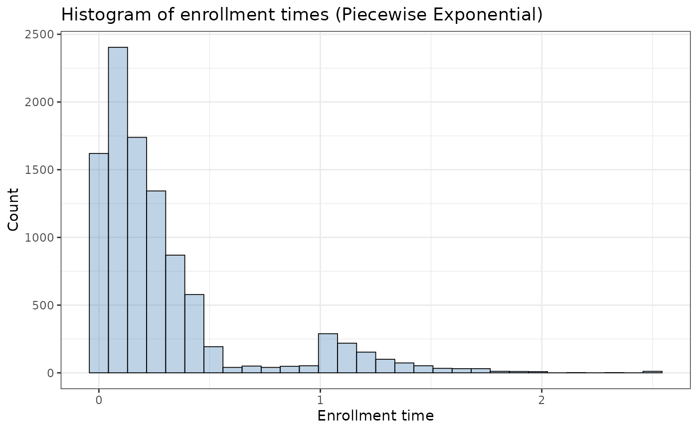

For transparency, the sampler proceeds as follows:

• For each subject, it simulates the waiting time until enrollment, starting from time 0.
• It checks interval by interval: If a randomly drawn exponential waiting time (using the interval’s rate) falls within that interval, the subject enrolls at that time.
• If not, the process moves to the next interval (with its potentially different rate), adding the completed interval’s duration to the subject’s time.
• This repeats until enrollment occurs or the final cutpoint is reached.
• After the loop finishes (either by an enrollment event occurring or by reaching the end of all intervals), it ensures the subject’s enrollment time does not exceed the final defined cutpoint.

Piecewise Enrollment with Proportions

Assume a 24-month trial with a target enrollment of \(N = 1{,}100\) patients. Suppose we want the enrollment pattern to be:

• 10% enrolled during months 0–8,
• 35% enrolled during months 8–16, and
• 55% enrolled during months 16–24.

To achieve this piecewise exponential enrollment pattern, we solve for the exponential rates in each interval using basic probability.

First, set the cutpoints to define the three enrollment windows piecewise_enrollment_cutpoints = c(0, 8, 16, 24). This creates three time bins: \([0,8),[8,16)\), and \([16,24]\). Next, solve for \(\lambda_1\) so that \(10 \%\) of patients enroll before month 8. For an exponential waiting time in the first interval,

\[ P(T<8)=1-e^{-8 \lambda_1}=0.10 . \]

Rearranging,

\[\begin{align*} 1 - e^{-8\lambda_1} &= 0.10 \\ e^{-8\lambda_1} &= 0.90 \\ -8\lambda_1 &= \log(0.90) \\ \lambda_1 &= -\frac{\log(0.90)}{8}. \end{align*}\]

Second, solve for \(\lambda_2\) so that \(35 \%\) of patients enroll in the second bin (months \(8-16\) ). This probability is

\[ P(8 \leq T<16)=P(T \geq 8) P(T-8<8 \mid T \geq 8)=e^{-8 \lambda_1}\left(1-e^{-8 \lambda_2}\right)=0.35 . \]

Using \(e^{-8 \lambda_1}=0.90\), we get \[\begin{align*} 0.90\left(1 - e^{-8\lambda_2}\right) &= 0.35 \\ 1 - e^{-8\lambda_2} &= \frac{0.35}{0.90} \\ e^{-8\lambda_2} &= 1 - \frac{0.35}{0.90} \\ \lambda_2 &= -\frac{1}{8}\log\left(1 - \frac{0.35}{0.90}\right). \end{align*}\] The third rate, \(\boldsymbol{\lambda}_3\), does not affect the overall proportion enrolled in months 16-24 (that remaining \(55 \%\) is already determined by \(\lambda_1\) and \(\lambda_2\) ). However, \(\lambda_3\) does affect the shape of the enrollment-time distribution within the final bin, here we set this value to 0.25.

Putting this together:

# define rates from calculations above
rate1 <- -log(.9)/8
rate2 <- -log(1-.35/exp(-rate1*8))/8
  

pw_example2 <- makeData(
  correlation_matrix    = NULL,
  sample_size_per_group = 5000,
  SEED = 321,
  endpoint_details = list( 
    list(
      endpoint_type  = "tte",
      baseline_rate  = .0558,        
      trt_effect     = 0,   
      fatal_event    = TRUE)),
  enrollment_details = list(
    administrative_censoring = 24,
     enrollment_distribution = "piecewise",
    piecewise_enrollment_cutpoints = c(0, 8, 16, 24),
  piecewise_enrollment_rates  = c(rate1, rate2, .25)
  ),
  non_fatal_censors_fatal = FALSE
)

And to double check enrollment scheme:

pw_example2$data %>%
    dplyr::summarize(.,
  Bin1 = mean(enrollTime < 8),
  Bin2 = mean(enrollTime >= 8 & enrollTime < 16),
  Bin3 = mean(enrollTime >= 16)
) %>% knitr::kable(.,caption="Observed enrollment proportion by time period")

Observed enrollment proportion by time period

Bin1	Bin2	Bin3
0.107	0.3471	0.5459

References

Cario, M. C., & Nelson, B. L. (1997). Modeling and generating random vectors with arbitrary marginal distributions and correlation matrix (pp. 1-19). Technical Report, Department of Industrial Engineering and Management Sciences, Northwestern University, Evanston, Illinois.